
AIAA 2004 - 3700 GUIDELINES FOR A SPACE PROPULSION DEVICE BASED ON HEIM'S QUANTUM THEORY
12/05/2014 22:54
AIAA 2004 - 3700
GUIDELINES FOR A
SPACE PROPULSION DEVICE
BASED ON HEIM'S QUANTUM THEORY
Walter Dröscher1, Jochem Häuser 1,2
1Institut für Grenzgebiete der Wissenschaft (IGW),
Leopold - Franzens Universität Innsbruck, Innsbruck, Austria
2Department of Transportation, University of Applied Sciences
and
Department of High Performance Computing, CLE GmbH, Salzgitter, Germany
40TH AIAA/ASME/SAE/ASEE
JOINT PROPULSION CONFERENCE & EXHIBIT, FORT LAUDERDALE, FLORIDA,
11-14 JULY, 2004
1 Senior scientist, 2 Senior member AIAA, member SSE, www.cle.de/HPCC, www.uibk.ac.at/c/cb/cb26/
The text of the calligraphy on the front page means Cosmos, comprising the two chinese symbols
for space and time. This calligraphy was done by Hozumi Gensho Roshi, Professor of Applied Sciences
at Hanazono University, Kyoto, Japan in September 2003. The two red squares depict the seal
of Hozumi Gensho Roshi.
2004
Institut für Grenzgebiete der Wissenschaft,
Leopold - Franzens Universität Innsbruck,
Innsbruck, Austria
Table of Contents
1 Space Propulsion and Higher-Dimension Quantized Spacetime Physics..........................................4
1.1 Basic Concepts of HQT ..........................................................................................................5
1.2 LQT and HQT............................................................................................................................6
1.3 Fundamental Physical Interactions in 8-D Quantized Space.................................................7
2 The Physical Principles for Field Propulsion ...................................................................................8
2.1 The Physics of Hermetry Forms................................................................................................8
2.2 The Metric for Electromagnetic Interactions...........................................................................10
2.3 The Metric for Coupling Electromagnetism and Gravitation..................................................11
2.4 Physical Model for Gravitophoton Generation.........................................................................13
2.5 Conversion of Photons into Gravitophotons............................................................................14
3 Space Flight Dynamics of Gravitophoton Field Propulsion...........................................................16
3.1 Gravitophoton Interaction Equations for Space Propulsion ...................................................16
3.2 Technical Data for Acceleration Gravitophoton Field Propulsion .........................................17
3.3 Space Flight in Parallel Space................................................................................................18
3.4 Lunar, Interplanetary, and Interstellar Missions......................................................................19
4 Cosmology from HQT and LQT ....................................................................................................20
4.1 Deficiencies in Current Fundamental Physical Theories.........................................................21
4.2 Common Concepts in HQT and LQT......................................................................................21
4.3 Cosmological Consequences...................................................................................................22
4.4 Dark Matter .............................................................................................................................23
4.5 Dark Energy.............................................................................................................................23
5 Conclusions and Future Work.........................................................................................................23
Acknowledgment.................................................................................................................................24
Appendix A: Mass Spectrum of Elementary Particles.......................................................................25
Appendix B: Gravitational Coupling Constants..................................................................................25
Glossary...............................................................................................................................................25
References...........................................................................................................................................28
Abstract
This paper is the third one in a series of publications,
describing a novel and revolutionary space
propulsion technique, based on a unified field
theory in a quantized, higher-dimensional space,
developed by the late B. Heim and the first
author, termed Heim quantum theory (HQT) in
the following. It is interesting to note that this
theory shares a similar physical picture, namely
a quantized spacetime, with the recently published
loop quantum theory (LQT) by L. Smolin,
A. Ashtektar, C. Rovelli, M. Bojowald et al. [11,
24-28]. LQT, if proved correct, would stand for
a major revision of current physics, while HQT
would cause a revolution in the technology of
propulsion.
For effective and efficient interplanetary as well
as interstellar travel, NASA's Breakthrough
Propulsion Physics Program (BPP) specified
three basic features, namely little or no fuel
mass, limited amount of energy consumption (a
spacecraft approaching the speed of light would
not satisfy this requirement, since its mass becomes
infinite), and (preferably) superluminal
speed. To satisfy these requirements a revolution
in space propulsion technology is needed.
Such breakthrough propulsion techniques can
only emerge from novel physics. If we believed
that current physics held the answer to all questions,
a BPP device would not be possible. Recently,
however, more and more evidence has
been piling up that current physics is far from final
answers and, in addition, exhibits fundamental
inconsistencies, even on the classical level.
Furthermore, quantum theory (QT) in its current
form does not lead to an explanation of the elementary
structures of matter, and does not lead
to a consistent cosmology either.
For a revolutionary space transportation system,
however, the physical concepts of matter and
inertia as well as the nature of space and time
have to be understood. In QT the existence of
matter is taken for granted, defining an elementary
particle as a point-like structure [17]. In
classical physics, including the General Theory
of Relativity (GR), science starts from the belief
that space and time are infinitely divisible, in
other words, that spacetime is continuous (a differentiable
manifold in the mathematical sense).
Both ideas contradict Nature's all pervading
quantization principle and immediately lead to
contradictions in the form of infinite self-energies
etc. or self-accelerations [18]. HQT is an
extension of Einstein's GR, using his field equations
as a template in a quantized higher-dimensional
space, but also extending these equations
into the subatomic range. This eventually leads
to a poly-metric, whose partial metric structures
are interpreted as fundamental physical interactions.
This theory, seems to complement both
QT and GR, in explaining the nature of elementary
particles as well as their discrete mass spectrum
and life times, based on the basis of a
quantized geometrodynamics (quantized elemental
surfaces of some 10-70m2, termed metron
by Heim) in a 12 dimensional space. Heim
derives a dimensional law that determines the
maximum number of possible dimensions that
can exist, along with admissible subspaces, and
also gives their physical interpretation. HQT
seems to be able to explain the nature of matter
(physicists deemed this question to be of importance
in the early fifties, see [21]). The physical
features of the postulated 12 dimensional, quantized
hyperspace, denoted as Heim space by the
authors, is described in detail. The 12D Heim
space comprises five semantic units, namely,
the subspaces ℝ3 (space), T1 (time), S2 (organization),
I2 (information), and G4 (steering of I2)
where superscripts denote dimension. Except for
the 3 spatial dimensions, all other coordinates
are imaginary. Several metric tensors can be
constructed from these subspaces. Each metric
tensor is associated with a specific physical interaction,
similar to Einstein's GR, where spacetime
curvature is interpreted as gravitation
(graviton). Analyzing the metric tensors acting
in ℝ4, the theory predicts six fundamental interactions,
instead of the four experimentally
known ones. These interactions represent physical
fields that are carrying energy. According to
HQT, a transformation of electromagnetic energy
into gravitational energy should be possible.
It is this interaction that is used as the physical
basis for the novel space propulsion concept,
termed field propulsion [1, 2], which is not
conceivable within the framework of current
physics.
1
The paper comprises four technical chapters. In
the first chapter, a qualitative discussion of the
six fundamental interactions, derived from the
concept of Heim space and its consequences for
a novel propulsion system, are presented. In addition,
a qualitative discussion of the physical
principle that serves as the basis for advanced
propulsion is given. In chapter two, the physical
principles of the so called field propulsion system
are quantitatively addressed, explaining
their application in future spaceflight2. In particular,
it is shown how the poly-metric from
Heim space leads to a metric describing electromagnetic
phenomena and its conversion into a
gravitational3 like metric, postulating a novel
particle, the gravitophoton. In chapter three, the
equations of the gravitophoton interaction are
derived, and a physical model is presented to
calculating the magnitude of the gravitophoton
interaction. This is also the main chapter, presenting
the quantitative physical model of the
gravitophoton interaction and the concept of
parallel space from which the physical guidelines
for the field propulsion device can be derived.
In particular, the technical requirements
for a gravitophoton propulsion device will be
discussed. The experimental set up of such a device
will also be presented. In addition, a lunar
mission, an interplanetary, and an interstellar
mission will be investigated. In chapter four,
similarities between HQT and LQT are discussed.
Cosmological consequences dealt with
concern the amount of dark matter (concept of
parallel space) and the cause of dark energy. The
acceleration of the cosmic expansion is explained
qualitatively, since it turns out that the
postulated sixth fundamental force (interpreted
as quintessence) and represented by the postulated
vacuum particle, is of repulsive nature.
Nomenclature and physical constants
à value for the onset of conversion of photons
into gravitophotons, see Eq. (39).
2 This chapter contains a certain amount of mathematics.
The reader may wish to skip the derivations and
continue with the gravitational Heim-Lorentz force,
Eq. (47).
3 The term gravitational is reserved to the two additional
interactions represented by the gravitophoton
and the vacuum particle acting on material particles.
A denotes the strength of the shielding potential
caused by virtual electrons, see Eq. (37).
Compton wave length of the electron
¤C= h
me c
=2.43×10⁻¹²m, ƛC=¤C /2¤.
c speed of light in vacuum 299,742,458 m/s ,
( 1/c2=¤0¤0 ).
D diameter of the primeval universe, some 10125
m, that contains our optical universe.
DO diameter of our optical universe, some 1026
m.
d diameter of the rotating torus, see caption Table
.
dT vertical distance between magnetic coil and
rotating torus (see Fig.1).
-e electron charge -1.602 × 10⁻¹⁹ C.
e¤z unit vector in z-direction.
Fe electrostatic force between 2 electrons.
Fg gravitational force between 2 electrons.
Fgp gravitophoton force, also termed Heim-Lorentz
force, Fgp=¤p e¤0 vT×H , see Eq. (47).
G = Gg + Ggp + Gq = 6.67259 × 10⁻¹¹ m3 kg-1 s-2,
gravitational constant .
Gg graviton constant, Gg≈G that is Gg decribes
the gravitational interaction without the
postulated gravitophoton and quintessence interactions.
Ggp gravitophoton constant, Ggp≈¤1/67¤2Gg .
Gq quintessence constant, Gq≈4×10⁻¹⁸Gg .
gi k
¤ gp¤ metric subtensor for the gravitophoton in
subspace I2∪S2 (see glossary for subspace description).
gi k
¤ ph¤ metric subtensor for the photon in subspace
I2∪S2∪T1 (see glossary for subspace description).
2
h Planck constant 6.626076 × 10⁻³⁴ J¤s,
ℏ=h/2¤.
hik metric components for an almost flat spacetime.
ℓ p= ¤Gℏ3
c3 =1.6×10⁻³⁵m Planck length.
me electron mass 9.109390 × 10⁻³¹ kg.
m0 mass of proton or neutron
1.672623 × 10- 27 kg and 1.674929 × 10⁻²⁷ kg.
Nn number of protons or neutrons in the universe.
q electric charge.
R distance from center of coil to location of
virtual electron in torus, see Fig.(1).
rN distance from nucleus to virtual electron in
torus, see Fig.(1).
R_ is a lower bound for gravitational structures,
comparable to the Schwarzschild radius.
The distance at which gravitation changes sign,
ρ, is some 46 Mparsec.
R+ denotes an upper bound for gravitation and
is some type of Hubble radius, but is not the radius
of the universe, instead it is the radius of
the optically observable universe. Gravitation is
zero beyond the two bounds, that is, particles
smaller than R- cannot generate gravitational interactions.
re classical electron radius
re= 1
4¤¤0
e2
me c2=3 × 10⁻¹⁵m.
rge ratio of gravitational and electrostatic
forces between two electrons.
v velocity vector of charges flowing in the magnetic
coil, see Eq. (27), some 103 m/s in circumferential
direction.
vT bulk velocity vector for rigid rotating ring
(torus) (see Sections. 3 and 4), some 103 m/s in
circumferential direction.
wgp probability amplitude (the square is the coupling
coefficient) for the gravitophoton force
(fifth fundamental interaction)
wgp
2 =Ggp
me
2
ℏ c
=3.87×10−49 probability amplitudes
(or coupling amplitudes) can be distance dependent
(indicated by a prime in [9]).
wgpe probability amplitude for emitting a gravitophoton
by an electron
wgpe=wgp .
wgpa probability amplitude for absorption of a
gravitophoton by a proton or neutron
wgpa
2 =Ggpmp
me
ℏ c
.
wg_q conversion amplitude for the transformation
of gravitophotons and gravitons into the
quintessence particle, corresponding to the dark
energy (rest mass of some 10-33 eV).
wph probability amplitude (the square is the
coupling coefficient for the electromagnetic
force, that is the fine structure constant α)
wph
2 = 1
4¤¤0
e2
ℏ c
= 1
137
.
wph_qp conversion amplitude for the transformation
of photons into gravitophotons (see Eq.
(35)).
wq probability amplitude for the quintessence
particle,(sixth fundamental interaction), corresponding
to dark energy (rest mass of some 10- 33
eV).
Z atomic number (number of protons in a nucleus
and number of electrons in an atom)
Z0 impedance of free space,
Z0=¤¤0
¤0
≈376.7¤.
α coupling constant for the electromagnetic
force or fine structure constant 1/137.
αgp coupling constant for the gravitophoton
force .
3
γ ratio of probabilities for the electromagnetic
and the gravitophoton force
¤=¤wph
wgp ¤2
=1.87×1046 .
¤0 permeability of vacuum 4π × 10-7 N/m2 .
¤ metron area (minimal surface 3Gh/8c3),
current value is 6.15 x 10-70 m2.
Φ gravitational potential, =GM/R.
ω rotation vector (see Fig. 1 ).
Abbreviations
BPP breakthrough propulsion physics
GR General Relativity
HQT Heim Quantum Theory
LQT Loop Quantum Theory
LHS left hand side
ls light second
ly light year
QED Quantum Electro-Dynamics
RHS right hand side
SR Special Relativity
VSL Varying Speed of Light
Subscripts
e electron
gp gravitophoton
gq from gravitons and gravitophotons into quintessence
ph denoting the photon or electrodynamics
sp space
Superscripts
em electromagnetic
gp gravitophoton
ph photon
T indicates the rotating ring (torus)
Note: Since the discussion in this paper is on
engineering problems, SI units (Volt, Ampere,
Tesla or Weber/m2 ) are used. 1 T = 1 Wb/m2 =
104 G = 104 Oe, where Gauss (applied to B, the
magnetic induction vector) and Oersted (applied
to H, magnetic field strength or magnetic intensity
vector) are identical. Gauss and Oersted are
used in the Gaussian system of units. In the
MKS system, B is measured in Tesla, and H is
measured in A/m (1A/m = 4π × 10-3 G). Exact
values of the physical constants are given in
[22].
Note: For a conversion from CGS to SI units,
the electric charge and magnetic field are replaced
as follows:
1 Space Propulsion and Higher-Dimension
Quantized Spacetime Physics
For effective and efficient lunar space transportation
as well as interplanetary or even interstellar
space flight a revolution in space propulsion
technology is needed.
Regarding the requirements of NASA's Breakthrough
Physics Propulsion Program (BPP) a
revolutionary space propulsion system should
• use no or a very limited amount of fuel,
• possibility for superluminal speed, and
• requirement for a low energy budget. This
immediately rules out any device flying close
to the speed of light, since its mass is going to
infinity, according to SR. A spacecraft having
a mass of 105 kg, flying at a speed of 1% of
the speed of light, carries an energy content
of 4.5x10¹⁷ J. Even if the spacecraft can be
provided with a 100 MW nuclear reactor, it
would take some 143 years to produce this
amount of energy.
It is understood that the laws of current physics
do not allow for such a revolutionary space propulsion
system. Propulsion techniques of this
4
e¤e/¤4¤¤0 and H¤¤4¤¤0H.
type can only emerge from novel physics, i.e.,
physical theories that deliver a unification of
physics that are consistent and founded an basic,
generally accepted principles, either removing
some of the limits, or giving rise to additional
fundamental forces, and thus providing alternatives
to current propulsion principles. Theories
like HQT and LQT are therefore of great interest,
since they might offer the potential for these
advanced technologies, see, for instance, the remark
on p. 9 in [29].
Hopes for such a unified theory are, indeed, not
futile. In classical physics, science starts from
the belief that space, time, and matter are infinitely
divisible, in other words, that spacetime is
continuous (a differentiable manifold in the
mathematical sense) and not subjected to the
quantization principle. Regarding the microcosm,
there exists a large number of elementary
particles that cannot be subdivided any further.
In quantum physics arbitrary divisibility of matter
has proved to be an illusion. On the other
hand, the existence of matter is taken for
granted, i.e., the occurrence of elementary particles
is accepted as such, and the cause for the
existence of matter cannot be revealed. There is
substantial evidence that the currently favored
Standard Model is far from being the final theory.
In the twentieth century there has been enormous
progress in physics, based on both Einstein's
theory of general relativity and quantum
theory. Both theories are very successful in their
own range, but could not be unified so far. The
reason for the unification is ... Despite the
successes of the two theories, the current status
of physical theory lacks the understanding of the
most fundamental physical facts. First, it has not
been possible, despite numerous attempts over
the last eight decades, to extent Einstein's idea
beyond the range of gravitation. Second, QT has
not been able to deliver the mass spectrum of
elementary particles, nor is there a theoretical
explanation for their lifetimes, neither can quantum
numbers be derived. None of these theories
is able to explain the nature of matter and inertia,
topics that are essential for the physics of a
completely novel propulsion system.
1.1 Basic Concepts of HQT
Einstein's view was eventually deemed untenable,
because next to gravitation other forces became
known. The recent article by L. Smolin
[11] on Atoms of Space and Time, however,
seems to be a sign that physics may be returning
to the Einsteinian picture, namely the geometrization
of the physical world, meaning that
all forces (interactions) are ultimately determined
by the structure of spacetime. The two
important ingredients that Einstein did not use
are a discrete spacetime and a higher-dimensional
space, provided with special, additional
features.
It is known that the general theory of relativity
in a 4-dimensional spacetime delivers only one
possible physical interaction, namely gravitation.
Since Nature shows us that there exist additional
interactions, and because both GR and
the quantum principle are experimentally verified,
it seems logical to extend the geometrical
principle to a discrete, higher-dimensional
space. Consequently, Heim’s quantum theory,
HQT, of gravity and elementary structures of
matter is based on the geometric view of Einstein,
namely that geometry itself is the cause of
all physical interactions, but it uses the structure
of Einstein's field equations only as a template
for physical interactions in a higher-dimensional
discrete space, and extends them also to the microcosm.
Eventually developed by Heim and the first
author, the theory utilizes an 8-dimensional discrete
space4 in which a smallest elemental surface,
the so-called metron, exists. HQT, developed
first by Heim in the fifties and sixties, and
partly published in the following three decades
of the last century, seems to be compliant with
4 To be more precise, Heim's theory was extended from
6 to 8-dimensions by the first author and Heim, [7], to
obtain the unification of the four known interactions
(forces). In this process, it was found that two additional
gravitational like interactions should occur,
termed the gravitophoton field (attractive and repulsive)
and the vacuum field (repulsive, interpreted later
on as quintessence) [1, 7]. The dimensional law derived
by Heim requires a 12-dimensional space, but
the additional four coordinates are needed only in the
explanation of the steering of probability amplitudes
(information).
5
these modern requirements. It also makes a series
of predictions with regard to cosmology and
high energy physics [12] that eventually can be
checked by experiment.
Most important, however, Heim's extended theory
predicts two additional interactions [1, 6-
9] identified as quintessence, a weak repulsive
gravitational like interaction (dark energy) and
gravitophoton interaction, that enables the conversion
of electromagnetic radiation into a
gravitational like field, represented by the two
hypothetical gravitophoton (negative and positive
energies) particles. The gravitophoton interaction
is discussed in Chaps. [2, 3.1]. Quintessence
(dark energy) is briefly discussed in Chap.
[4].
The interpretation of the physical equations for
the gravitophoton field leads to the conclusion
that this field could be used to both accelerate a
material body and to cause a transition of a material
body into some kind of parallel space,
possibly allowing superluminal speed. These effects
could serve as the basis for advanced space
propulsion technology, and are dealt with quantitatively
in the following chapters.
According to Heim's theory, gravitation, as we
know it, is comprised of three interactions,
namely by gravitons, the postulated gravitophotons,
and by the quintessence particle. This
means that the gravitational constant G contains
contributions from all three fields. The quintessence
interaction, however, is much smaller than
the first two contributions.
It is interesting to note, that the mass spectrum
for elementary particles, calculated from Heim's
mass formula, and partly shown in Appendix A
as taken from [12], is very sensitive to G. A corrected
value of G obtained by the first author,
accounting for the contribution of the gravitophoton
field, led to substantially improved results
of the mass values when compared to experimental
data. In Heim's theory the existence
of matter as an independent entity is replaced by
the features of a dynamic 8-dimensional discrete
space, and as such is created by space itself. In
other words, matter is caused by a non-Euclidean
metric in space ℝ8, termed 8D Heim space,
comprised by a large number of elemental space
atoms (called metrons by Heim), interacting in a
dynamic and highly complex way.
A few words about the history of HQT seem to
be in place. Heim first published his theory of a
higher-dimensional discrete spacetime in an obscure
German journal [10] in a series of four articles
in 1959. In 1977, following the advice of
Heisenberg’s successor, H.-P. Dürr, Heim published
an article entitled Vorschlag eines Weges
zur einheitlichen Beschreibung der Elementarteilchen
(Recommendation of a Way to a Unified
Description of Elementary Particles) [4],
which in today's terminology was a summary of
his theory for a unified field theory including
quantum gravity. Later on, he wrote two text
books Elementarstrukturen der Materie [6, 7]
that were eventually published by A. Resch (see
Acknowledgment). However, to be fair, it
should be mentioned that Heim's publications
are difficult to read, and needed to be modified
and extended by the first author in several ways,
for instance [9].
1.2 LQT and HQT
In order to understand how to categorize Heim's
quantum theory, it seems worthwhile to determining
the similarities between recent loop
quantum theory by L. Smolin, A. Ashtekar, and
C. Rovelli [11, 24, 25] and HQT, and also to
learn how HQT compares with GR and QT. A
major difference between GR and Heim is that
in GR the material field source does not appear
in geometrized form, but occurs as a phenomenological
quantity (in the form of matter that is
an entity of its own, whose existence is taken for
granted).
It should be noted that HQT complements both
QT and GR, in explaining the nature of elementary
particles as well as their discrete mass spectrum
and life times, based on the basis of a
quantized geometrodynamics (quantized elemental
areas of some 10-70 m2, termed metron
by Heim) in a 12 dimensional space (3 real and
9 imaginary coordinates). As shown by Heim
the fact that all additional coordinates are imaginary
leads to real eigenvalues in the mass spectrum
for elementary particles [4, 6]. The idea of
geometrization is extended to the sub-atomic
range. However, in that case, the Christoffel
6
symbols need to be replaced by real tensor components5.
Heim derives a dimensional law that
restricts the maximum number of dimensions to
12 and requires the existence of subspaces.
From the metric of subspace ℝ6, originally conceived
by Heim, the premises of QT cannot be
derived, and the quantization principle had to be
introduced ad hoc. For instance, Dirac's equations
cannot be derived within ℝ6. However,
when the metric in space ℝ8 is considered, all
possible physical interactions are reproduced.
The complete space ℝ12 is needed to explain
how probability amplitudes (immaterial) are
steering events in spacetime ℝ4.
In the following, a Heim space is a quantized
space comprising elemental surfaces with orientation
(spin), the metron, whose size is the
Planck length (apart from a factor) squared,
comprising 6, 8, or 12 dimensions. A Heim
space may comprise several subspaces, each
equipped with its individual Riemannian metric.
The union of these individual metric spaces is
termed a poly-metric.
Furthermore, in GR the gravitational potential
is associated with the metric tensor, and thus
has a direct physical meaning. Extending this
concept to the poly-metric in Heim space ℝ8,
and forming special combinations of these partial
metrics, all possible fundamental physical
interactions are obtained. Since GR has been extremely
well verified experimentally, this interpretation
seems to be justified.
1.3 Fundamental Physical Interactions in
8-D Quantized Space
In GR the gravitational force is nothing but an
effect of the geometric curvature of spacetime.
The predictions of GR have been tested extensively,
and today GR arguably is the experimentally
best verified theory. Therefore, there is
some confidence that this concept can be extended
to all physical forces, and that the structure
of the equations of GR is valid for all physical
interactions in a higher-dimensional space.
5 This can be shown by employing the double transformation
described in Eq. (2) to Heim's eigenvalue
equations for the mass spectrum of elementary particles.
Otherwise masses of particles could be transformed
away which is unphysical.
A Heim space ℝ12, where the superscript denotes
dimension, comprises five subspaces or partial
structures that form semantic units. Combining
these semantic units by employing certain selection
rules a set of so called hermetry forms or
partial metric tensors is obtained, forming the
poly-metric, that represents all physical interactions
[2]. Each of the semantic units (or subspaces)
has its own metric. There are the subspaces
ℝ3 with real coordinates (x1, x2, x3), T1
with imaginary time coordinate (x4), S2 with
imaginary coordinates for organization of structures
(x5, x6,), I2 with imaginary coordinates for
information (x7, x8), and G4 with imaginary coordinates
for steering of probality amplitudes and
thus events in ℝ4 (x9, x10, x11, x12). The space ℝ12
is comprised of the two spaces ℝ6 = ℝ3∪T1 ∪S2
and V6 =I2 ∪G4. The concept of energy exists in6
ℝ6, while V6 is denoted as immaterial. Considering
the space ℝ8 = ℝ3∪T1∪S2∪I2, that is omitting
the space G4, the theory predicts six fundamental
interactions, instead of the four experimentally
known ones. These interactions emerge
in our spacetime and represent physical fields
carrying energy. According to the theory, a
transformation of electromagnetic energy into
gravitational energy (gravitophoton) should be
possible (see Chap. 2.5). It is this conversion
that is used as the physical basis for the novel
space propulsion concept [1, 2], which is not
conceivable within the framework of current
physics. This is a direct consequence of the dimension
of Heim space, and the interpretation of
a partial metric (hermetry form, see glossary) as
a physical interaction or particle. In other words,
if Einstein's view, namely of geometry being the
cause of gravitation is extended to the poly-metric
in Heim space, the interpretation of all physical
interactions is a natural consequence. Moreover,
the two additional interactions should also
be considered real.
It seems that space G4 does not have a direct
physical meaning in a sense that it is responsible
for physical interactions. Its role seems to be
acting as a symmetry breaking principle, respon-
6 This is not completely correct, since the vacuum or
quintessence particles of hermetry form H10(I2) (see
glossary and [2]) with I2⊂ℝ8 possess (small) energies.
7
sible for a quantized bang, and much later on
(some 1010 years ago), for the creation of matter.
Starting from Einstein's equations, Heim derives
a set of nonlinear eigenvalue equations for microscopic
particles (mass spectrum of elementary
particles), first in ℝ6. In Heim”s theory,
quantum mechanics is not contained in ℝ6, but
in space ℝ8. In this regard, Heim's theory can be
understood as being complementary to the wave
picture, taking care of the particle nature of
physical objects (see [7] pp. 360 for the linear
Dirac equations.
2 The Physical Principles for Field
Propulsion7
In the following a roadmap for the derivation of
the gravitophoton interaction is presented.
The proposed propulsion concept works in two
stages. First, a gravitophoton field is generated
through interaction with an electromagnetic field
that exerts a force on the space vehicle. Second,
there exist parallel spaces in which covariant
laws of physics are valid that allow speeds
larger than the vacuum speed of light in ℝ4. Under
certain conditions, a spacecraft can enter a
parallel space, see Sec. (3.3).
For the gravitophoton interaction to exist, Einstein's
principle of geometrization of physics
needs to be valid for all physical interactions.
According to HQT this is the case in 8D space.
For instance, in classical physics, there is no difficulty
to include electromagnetism in general
relativity by adding the stress-momentum-tensor
of the electromagnetic field Ti k
em to the RHS of
Einstein's field equations in 4D spacetime
Ri k=¤¤Ti k
g ¤Ti k
em−1
2
gi k T ¤ (1)
and T=Tk
k contains both the gravitational and
electromagnetic contribution. The parameter κ is
7 The term breakthrough propulsion is not used, since it
does not relate to the propulsion principle that is based
on the conversion of photons (electromagnetic field)
into gravitophotons (gravitational like field).
of the form ¤=
8¤G
c4 . To complete the set of
equations, Maxwell's equations have to be
added. This is, however, not the approach of a
unified field theory, because the electrodynamic
field is added from the outside without any geometrical
interpretation. In the next section, the
concept underlying the unification of all physical
interactions is derived, extending Einstein's
principle of geometrization.
2.1 The Physics of Hermetry Forms
As described in [1] there is a general coordinate
transformation xm¤¤¤¤¤i ¤¤ from
ℝ4¤ℝ8¤ℝ4 resulting in the metric tensor
gi k=
∂ xm
∂¤¤
∂¤¤
∂¤i
∂ xm
∂¤¤
∂¤¤
∂¤k
(2)
where indices α, β = 1,...,8 and i, m, k = 1,...,4.
The Einstein summation convention is used, that
is, indices occurring twice are summed over.
The above transformation is instrumental for the
construction of the poly-metric used to describing
physical interactions. The Euclidean coordinates
xm and curvilinear coordinates ¤i are in ℝ4,
while curvilinear coordinates ¤¤ are in ℝ8. The
metric tensor can be written in the form
gi k=: Σ
¤,¤=1
8
gi k
¤¤¤¤
(3)
and the individual components are given by
gi k
¤¤¤¤=
∂ xm
∂¤¤¤¤
∂¤¤¤¤
∂¤i
∂ xm
∂¤¤¤¤
∂¤¤¤¤
∂¤k
. (4)
Parentheses indicate that there is no index summation.
In [2] it was shown that 12 hermetry
forms (see glossary) can be established having
direct physical meaning, involving specific combinations
from the four subspaces. The following
denotation for the metric describing hermetry
form Hℓ with ℓ=1,...,12 is used:
gi k ¤Hℓ ¤=: Σ
¤,¤∈Hℓ
gi k
¤¤¤¤
(5)
where summation indices are obtained from the
definition of the hermetry forms. The expres-
8
sions gi k ¤Hℓ ¤ are interpreted as different
physical interaction potentials caused by hermetry
form Hℓ, following the interpretation employed
in GR. The combination of coordinates
¤¤ and ¤¤ are characteristic for the interaction,
and also characterize the subspace. Applying the
sieve operator formed from Kronecker symbols,
namely
s ¤¤0 ,¤0¤:=¤¤0¤¤¤0¤ (6)
to Eq. (5) selects the term gi k
¤¤0¤0¤ . A sieve operator
(or sieve transformation) can be applied
repeatedly, and thus serves to convert one hermetry
form into another one. At the moment a
sieve operator is a mathematical construction
only, but it is the aim of this discussion to show
how such a conversion can be obtained in physical
reality. For the sake of simplicity, the following
short form, omitting subscripts ik, is introduced
¤¤¤¤:=gi k
¤¤¤¤ .
Next the hermetry forms pertaining to the three
subspaces S2 , I2, S2 × I2 are investigated. Cosmological
data clearly show that the universe is
expanding, which indicates a repulsive interaction.
Gravitational attraction is well known
since Newton. Both interactions act on matter,
so that there should be two hermetry forms having
anti-symmetric properties. The spaces corresponding
to these interaction are identified as S2
and I2. The gravitational field, as described by
gravitons, is given by hermetry form H12
gi k ¤H12¤=¤55¤¤¤56¤¤¤65¤¤¤66¤, (7)
while the vacuum field (quintessence) is given
by
gi k ¤H10¤=¤77¤¤¤78¤¤¤87¤¤¤88¤. (8)
There is a third hermetry form whose metric is
in the space S2× I2. Since this metric is a combination
of an attractive and a repulsive interaction,
it is assumed that there are exist two fields.
The first partial metric is considered to be attractive,
since its components contain the gravitational
metric of Eq. (7). For the same reason the
second part is considered to be repulsive. The
particle for mediating this interaction is called
the gravitophoton because of the possible interaction
with the electromagnetic field. The reasons
will become clear in the next section. It is
postulated from the metrics of Eqs.(9, 10) that
there are two types of gravitophotons associated
with the attractive and the repulsive gravitophoton
potentials. Their respective coupling constants
are denoted by Ggp
- and Ggp
+ that will
be described below. The attractive gravitophoton
particle is described by Eq. (9), the minus
sign denoting negative energy density, because
it contains the metric of the graviton which is directly
visible from Eq. (7). The repulsive gravitophoton
particle is described by Eq. (10), the
plus sign denoting positive energy density, because
it contains the metric of the vacuum or
quintessence particle that describes a repulsive
force. Their partial metric have the form
gi k ¤H11
- ¤=¤55¤¤¤56¤¤¤65¤¤¤66¤+
¤57¤¤¤67¤¤¤58¤¤¤68¤ (9)
gi k ¤H11
+ ¤=¤77¤¤¤78¤¤¤87¤¤¤88¤+
¤75¤¤¤76¤¤¤85¤¤¤86¤. (10)
To conclude this section, it has been shown that
in Heim space ℝ8 there are three physical interactions
acting on material particles, namely,
gravitation represented by hermetry form H12
(S2) (attractive), the quintessence or vacuum
field hermetry form H10 (I2) repulsive), and the
gravitophoton field, hermetry form H11 (S2, I2)
(both attractive and repulsive). Negative and
positive gravitophotons are generated simultaneously
in pairs, and H11 is the only hermetry form
that is identically 0, that is
gik ¤H11¤=gik ¤S2×I 2¤=0. (11)
It is a strange fact that a hermetry form that is
zero should have any physical effect at all. This
reflects the fact that the total energy being extracted
from the vacuum by pair production of
gravitophotons is zero. However, the physical
effect lies in the different absorption coefficients
of negative and positive gravitophotons. As it
turns out in Chap. 3, gravitophotons are generated
by virtual electrons, that is, they are gener-
9
ated by vacuum polarization 8. In this process
energy is conserved, but two different types of
energy both negative and positive are obtained,
adding up to zero. H11 is the only hermetry form
that is comprised by space S2× I2, the so called
transcoordinates9. No other of the hermetry
forms is identical to 0, since this is the only hermetry
form associated with creating particles
from the vacuum.
Hence, the gravitational constant G is comprised
of the three individual coupling strengths of
these interactions
G=Gg¤Ggp¤Gq (12)
where10 Ggp≈1/672Gg and Gq≈4×10⁻¹⁸Gg .
In the following section the metric describing
photons, given by hermetry form H5 (T1, S2, I2),
and its interaction with the gravitophoton metric
is investigated.
2.2 The Metric for Electromagnetic Interactions
The metric tensor for photons depends on subspaces
I2, S2, and T1 with coordinates ¤4, ¤5,...,¤8,
see [2].
gi k
¤ ph¤ :=gi k ¤H5¤= Σ
¤,¤=4
8
gi k
¤¤¤¤
(13)
The coupling constant of this hermetry form is
¤=wph
2 = 1
4¤¤0
e2
ℏ c
.
8 A nonzero vacuum density during the early universe
resulted in an exponential expansion (inflationary
phase), and also is the cause of the Casimir effect, although
extremely small. GR alone cannot provide the
physics for field propulsion. Moreover, vacuum energy
is also considered to be responsible for the expansion
of the universe.
9 Coordinates of S2 are associated with GR and those of
I2 are assigned to QT.
10 In the physical interaction picture, generally the first
partner emits and the second one absorbs a messenger
particle. Since the quintessence is formed from the
vacuum itself, there is no generating mass, for instance,
a proton mass emitting a photon. Thus the
value Gq is some kind of fictitious value.
For weak electrodynamic and also for weak
gravitational fields, spacetime (4D) is almost
flat, so one obtains
gi k=gi k
¤0¤¤hi k where g4 4
¤0¤=−1 and gi i
¤0¤=¤1
where i=1,2,3 and k, =1,...,ℓ 4. The hik are small
quantities whose products are negligible. In the
following the hik are used to describe the metric
for electromagnetic interactions. All other components
are 0. The geodesic equation [1] takes
the form
¨xi=−1
2 ¤∂hil
∂¤k
−
∂ hkl
∂¤i
¤
∂ hik
∂¤l ¤˙xk ˙xl .
where the dot denotes the time derivative.
Evaluating the terms on the RHS gives
−2 ¨xi=¤2 hi4 , 4−h44, i¤ ˙x4 ˙x4 +
2¤hi4 , l¤hil , 4−h4 l , i¤ ˙x4 ˙xl +
¤hik , l¤hil , k−hkl , i¤ ˙xk ˙xl .
(14)
with i,k,ℓ=1,2,3 and the comma denoting a partial
derivative. Investigating the first two terms
of Eq. (14) and using x4=ct 11 one obtains
¨xi=¤ 1
2
h44,i−hi4 , 4¤c2¤¤h4 l , i−hi4 , l ¤c ˙xl .
(15)
Introducing the quantity
Mi k=¤ 1
1¤¤k 4
hk 4, i – hi 4, k ¤,
Eq. (15) can be written in shortform
¨xi=Mik c ˙xk . (16)
This form can be directly compared with an
electron moving in an electromagnetic field
¨xi= e
me c
Fik ˙xk
(17)
where Fik=
∂ Ai
∂ xk−
∂ Ak
∂ xi and no distinction
needs to be made between covariant and the or-
11 It should be noted that in this section contravariant coordinates
are used.
10
dinary derivative. The electromagnetic field tensor
is obtained from the 4-vector electromagnetic
potential that is defined as ¤¤, Ai¤. From
comparison of Eqs. (16) and (17) the following
expression for the metric is obtained
h4 k= e
me c2 ¤1¤¤4 k ¤Ak .
(18)
In the next step, the third term of Eq. (14) is investigated.
Tensor potentials hi k can be written,
see [1], by means of retarded potentials
hi k= 1
4¤¤0
eQ
me c2 r
vi
c
vk
c
= e
me c2 Ai
˙xk
c (19)
with i, k=1,2,3. Combining Eqs. (17) and (18)
with Eq. (19), one obtains
hi k= 1
4¤¤0
¤1¤¤4 i¤4 k ¤ eQ
me c2 r
vi
c
vk
c (20)
with i, k =1,...,4.
Analyzing Eq. (20) shows that for i=4 and k=4
the metric describes the electric potential ¤,
while for k=4 and i=1,2,3 the metric represents
the vector potential A. For indices i, k=1,2,3
an additional tensor potential is obtained, which
is not present in classical electrodynamics.
Therefore, a 4×4 matrix is needed to describe all
electromagnetic potentials.
Tensor potentials hik with i, k =1,2,3 are belonging
to the hermetry form for photons and
thus have coupling coefficient ¤=wph
2 , but
cannot be associated with the 4-potential of the
electromagnetic field. Introducing the coupling
coefficient α in Eq. (20) leads to
hi k=¤¤1¤¤4 i¤4 k ¤Q
e
ℏ
me c
1
r
vi
c
vk
c
. (21)
On the other hand, hik= Σ
¤,¤=4
8
hi k
¤¤¤¤ is defined
by its sum of partial potentials, so that the sum
of all of these potentials is determining the coupling
constant for the electromagnetic field,
namely wph. Coupling constants for different
fields are thus determined by the corresponding
sum of their partial potentials.
2.3 The Metric for Coupling Electromagnetism
and Gravitation
As was shown above, the metric tensor for the
gravitophoton depends on subspaces S2 and I2
with coordinates ¤5, ¤6, ¤7, ¤8, and is written as
gi k
¤gp¤ :=gi k ¤H11¤= Σ
¤ ,¤=5
8
gi k
¤¤¤¤=0.
(22)
In comparison with Eq. (8), the metric for the
photon can be written in the form12
gi k
¤ ph¤=gi k
¤gp¤¤gi k
¤4 4¤¤ Σ
¤ , ¤=5
8
¤gi k
¤¤4¤¤gi k
¤4 ¤¤¤. (23)
The second and third terms, as will be shown
below, can be associated with the electric force
(electric scalar potential) and the Lorentz force
(vector potential). The first term represents the
combined metric for the negative and positive
gravitophoton particles. If an experiment can be
conceived which causes the metric of the photon
to become 0, then the metric for the gravitophoton
particles remains. The experiment needs to
remove the time dependence from the photon
metric, so that only the space S2 × I2 remains, responsible
for the gravitophoton metric 13.
In addition it can be shown, see Eq. (35), that in
the presence of virtual electrons, responsible for
the vacuum polarization and the shielding of the
charge of a nucleus [16], there exists a nonzero
probability amplitude for converting a photon
into gravitophotons. This gravitational force is
the basis for the propulsion concept, termed
gravitophoton field propulsion or field propulsion.
12 The sum of the second and third terms were denoted
as electromagnetic metric tensor, gi k
¤em¤ , in [1].
13 We are aware of the fact that these theoretical predictions
sound highly speculative, but they are direct consequence
of the geometrization principle.
11
For weak gravitational fields, spacetime is almost
flat, so the contribution of
∂¤4
∂¤4
is large in
comparison to
∂¤4
∂¤l
, l=1, 2,3. Therefore, only
the scalar photon potential needs to be considered
g4 4
¤ ph¤=g4 4
¤0¤¤h4 4
¤ ph¤ . (24)
For the linearized potential a formula similar to
Eq. (23) holds,
h4 4
¤ ph¤=h4 4
¤4 4¤+ Σ
¤ , ¤=5
8
¤h4 4
¤¤4¤¤hi k
¤4 ¤¤¤
+ Σ
¤, ¤=5
8
h4 4
¤¤¤¤ .
(25)
Next, the contributions of the partial potentials
on the RHS of Eq. (25) are evaluated. From the
known form of the electric and Lorentz forces,
F=q E¤q vT×B, vT denoting the velocity
of the rotating torus, there follows the existence
of a scalar electric potential ϕ and a vector potential
A with components Ai=¤0
Qvi
R
where
Qvi denotes the total current in the magnetic coil
and i=1,2,3. The first term in (25) is associated
with the electric potential, seen by a virtual electron
with charge -e at distance rN from a nucleus,
located in the torus, see Fig. (1). The potential
thus takes the form
h4 4
¤4 4¤=− 1
4¤¤0
1
me c2
eZe
rN
. (26)
For the first stage of the proposed propulsion
mechanism as well as for the experiment of Fig.
(1), it can be assumed that speed vi << c. No
field propulsion system will accelerate a spacecraft
to a velocity comparable to the speed of
light, since the required energy renders such an
approach impractical.
The second partial potential can be determined
from Eq. (19). The corresponding vector potential
is of the form
Σ
¤ ,¤=5
8
¤h4 4
¤¤4¤¤h4 4
¤4 ¤¤¤=− 1
4¤¤0
1
me c2
eQ
R
vi
c
vi
T
c (27)
with summation over i=1,2,3 and vi /c and Q the
speed and total charge of the electrons in the
current loop (see Fig. (1)), while vi
T /c denotes
a velocity component of the rotating torus (see
Fig. (1)). The charge -e denotes electron charge.
R is the distance from the center of the coil to
the location of a virtual electron in the torus.
This potential represents the Lorentz force.
There is a third partial potential in Eq. (25) that
has the form of a tensor potential, which has no
counterpart in classical electrodynamics theory
and comes from the geodesic equation. According
to the geometrization of forces, a new force
should exist, derived from
Σ
¤,¤=5
8
¤h4 4
¤¤¤¤¤=
− 1
4¤¤0
1
me c2
eQ
R
vi
c
vi
T
c
¤
vk
c
vk
T
c
¤
(28)
with summation over i and k, assuming values
1,2,3. The potential of Eq. (28) describes a scalar
potential that exists at a location in space carrying
a specific charge e/me. Adding up all three
contributions results in a potential
h4 4
¤ ph¤= 1
4¤¤0
1
me c2×
¤ eZ ¤r ¤e
r N
−eQ
R
vi
c
vi
T
c
−eQ
R
vi
c
vi
T
c
vk
c
vk
T
c
¤.
(29)
For distances r < rN, Z(r) is replacing Z, accounting
for the shielding effect of the charge of the
nucleus by the virtual electrons that are being
formed in the vicinity of a nucleus within the
range of the Compton wavelength of the electron.
It should be noted that the electron charge,
-e, was used in the first term. In the second and
third terms it should be noted that eQ > 0, since
electrons are involved. From Eq. (27) it is required
that the 4-dimensional vector potential,
(ϕ, Ai) with i=1,2,3, of classical electrodynamics
has to be replaced by the 4-dimensional tensor
potential (ϕ, Ai, Aik) with i,k =1,2,3. Since velocities
of charges in a material body are much
smaller than the speed of light, the value of the
12
factor vk /c vk
T /c being in the range of 10-11 to
10-16, it is understandable that the tensor potential
was not separately identified so far. Expressing
e Z ¤r ¤e=eZe¤eZe¤r ¤ where e(r) represents
the additional positive charge of the nucleus
resulting from the shielding effect of the
virtual electrons (see below), Eq. (29) takes the
form
h4 4
¤ ph¤= 1
4¤¤0
1
me c2×
¤ eZe
r N
¤eZ e
r N
−eQ
R
vi
c
vi
T
c
−eQ
R
vi
c
vi
T
c
vk
c
vk
T
c
¤.
(30)
Considering a nucleus of one of the atoms in the
material comprising the torus, there is a location
rN for which the first and third terms of Eq. (30)
cancel, namely for
rN=Z e
Q
R
c
vi
c
vi
T (31)
where the constant charge value Ze was used.
With e=Ae , see Eq. (35), the following equation
holds
eZe
r N
=AeQ
R
vi
c
vi
T
c
. (32)
The value of A, derived from vacuum polarization,
is specified in Eq. (36) and computed in
Eqs. (37, 38). If the value rN is smaller than
¤C= h
me c
=2.43×10⁻¹²m , the Compton wavelength
of the electron, the second term in (30) is
different from 0 and the speed vi can be chosen
such that the first and the third terms cancel,
leading to
h4 4
¤ ph¤= 1
4¤¤0
1
me c2
eQ
R
vi
c
vi
T
c
¤A−
vk
c
vk
T
c
¤. (33)
From the nature of A, it is obvious that the first
term in the above potential is generated from the
vacuum, wile the second term comes from the
tensor potential generated in the coil. The total
energy extracted from the vacuum is, however,
always zero. According to L. Krauss in [3] the
cosmological constant is 5×10⁻¹⁰ J/m3. This
means that the conversion of photons into gravitophotons
begins to occur as soon as the condition
h4 4
¤ ph¤≈0 is satisfied.
2.4 Physical Model for Gravitophoton Generation
In the following, starting from Eq. (33), the
physical mechanism is presented, responsible for
the conversion of photons into gravitophotons.
The mechanism for the generation of the postulated
negative and positive gravitophoton particles
is based on the concept of vacuum polarization
known from Quantum Electrodynamics
(QED). In QED the vacuum behaves like a dielectric
absorbing and producing virtual particles
and the Coulomb potential is associated
with the transfer of a single virtual photon. Vacuum
polarization in form of the electron-photon
interaction changes the Coulomb potential of a
point charge for distances within the electron
Compton wavelength with respect to a nucleus.
The velocities vi , vi
T in combination with the
total charge Q in the current loop or magnetic
coil need to be chosen such that
r N¤¤C , (34)
otherwise vacuum polarization does not occur. It
should be noted that the experiment allows to
vary these three parameters. However, as will be
shown below, two more conditions have to be
satisfied. In addition, the material in the torus
should contain hydrogen atoms to get a value of
Z as small as possible, that is close to 1.
A conversion of photons into gravitophotons is
possible according to Eqs. (35). The first equation
describes the production of N2 gravitophoton
particles14 from photons. This equation is obtained
from Heim's theory in 8D space in combination
with considerations from number theory,
and predicts the conversion of photons into
gravitophoton particles. The second equation is
taken from Landau [16]
14 The factor N2 results from the fact that in Eq. (35)
probability amplitudes are considered, but the generation
of particles depends on actual probabilities. It
should be noted that N is not needed, but the product
Nwgp.
13
wph ¤r ¤−wph=Nwgp
wph ¤r ¤−wph=Awph .
(35)
The physical meaning of Eqs. (35) is that an
electromagnetic potential containing probability
amplitude Awph can be converted into a gravitophoton
potential with associated probability amplitude
Nwgp. From Eqs. (35) the following relation
holds for gravitophoton production, requiring
the existence of a shielding potential
Nwgp=Awph . (36)
The function A(r) can be calculated from Landau's
radiation correction [16] and is given by
A= 2
3¤
¤∫
1
∞
e
−2
me c
ℏ
r ¤
¤1¤ 1
2 ¤2 ¤¤¤2−1¤1/2 /¤2 d ¤ (3
7)
with numerical values for A ranging from 10-3 to
10-4. For small r (r << λC) the integral in Eq.
(37) can be evaluated
A=−
2¤
3¤ ¤ln
me c
ℏ
r¤CE¤5
6 ¤ (38)
where CE = 0.577 is Euler's constant. For r >>
λC, the integral Eq. (37) falls off exponentially
as e
−2
me ℏ
c
r . Vacuum polarization changes the
Coulomb potential of a point charge only for
distances r < λC. The radiation correction is not
only caused by electron-positron interaction, but
interaction with muons and pions is also possible.
QED works for muons, but does not work
for pions, since they are subject to the strong interaction.
Therefore, for r ~ h/mπc, QED will not
suffice anymore, i.e., there is no applicable theory.
Hence, the physical model presented below
is limited to this fact.
The third condition is, according to Eq. (33), to
make the photon potential vanish, i.e., to trigger
the conversion of a photon into negative and
positive gravitophotons, which requires that A
takes on a value à that is
¤A
=
vk
c
vk
T
c
(39)
where the value of à depends on the velocities
of the charges in the coil and the rotating torus.
This conversion takes place at a larger value of
r, since the product on the RHS of Eq. (39) is
some 10-11.
2.5 Conversion of Photons into Gravitophotons
To summarize, there are the following three
conditions to be satisfied in order to convert a
photon into a pair of negative and positive gravitophotons
while insuring that the total energy
extracted in form of gravitophoton particles
from the vacuum is zero.
¤A
=
vk
c
vk
T
c
r N¤ ¤C= h
me c
r N=Z e
Q
R
c
vi
c
vi
T
(40)
The crucial point in the interpretation of Eq.
(40) is that the first equation provides a value of
Ã≈10-11. This value is needed to start converting
photons into gravitophotons. However, for this
value of à the conversion process is not efficient,
i.e., the number of gravitophotons produced
is too small to result in an appreciable
force. Equations two and three determine the
conditions at which, according to Eq. (42), an
effective gravitophoton potential exists for
which the respective value rN is determined. The
corresponding value for A > Ã is some 10-3. It
should be noted that Eq. (39) is not interpreted
as a resonance phenomenon, but sets a condition
for the photon potential to disappear and the
gravitophoton potential to appear that is, for the
onset of the conversion of photons into gravitophotons.
Once this happened, the value of A can
be increased further, giving rise to an efficient
and effective gravitophoton potential for field
propulsion15.
In the following these conditions will be employed
to determining the technical requirements
of a gravitophoton propulsion device.
Since an almost flat space was assumed, the
equation for the gravitophoton metric, Eq. (22),
15 It should be noted that this not a proof that the conversion
process takes place as indicated. Only the experiment
can prove the correctness of this assumption.
14
15
Figure 1: Instead of a simple current loop, a coil with many turns can be used. Both, the current in the coil and
the rotation are in counter-clockwise direction. The field of this coil gives rise to an inhomogeneous magnetic
field that has a radial field component. The radial component and the gradient in z-direction are related
through Hr=−r
2
∂Hz
∂z . It should be noted, however, that if the ring possesses a magnetic moment, M, there is
a magnetic force in the z-direction of magnitude F=M
∂Hz
∂ z . This force does not depend on the rotation of the
ring. For a diamagnetic material the force acts in the positive z-direction (up), while para- and ferromagnetic
materials are drawn toward the region of increasing magnetic field strength (down). The gravitophoton fore
superimposes these effects.
The gravitophoton force comes into play as soon as the ring starts rotating and the condition according to Eq.
(40) is satisfied. i.e., the velocity components vk and vk
Tmust have the same sign. Perhaps equipment used to
measuring magnetic moments can be employed to determine the gravitophoton force. For instance, if a paramagnetic
substance is used, the gravitophoton force (up) could be used to balance the magnetic force, so that
the resulting force is 0. From Refs. [23 and 24] it is found that a quartz sample (SiO2, diamagnetic) of a mass
of 10-3 kg experiences a force of 1.6 × 10⁻⁴ N in a field of Bz=1.8 T and a gradient of dBz/dz=17 T/m. A calcium
sample (paramagnetic) of the same mass would be subject to a force of -7.2 × 10⁻⁴ N. It is important
that the material of the rotating ring is an insulator to avoid eddy currents. For the acceleration phase, the
torus should contain hydrogen atoms. For transition into parallel space another material should be used.
¤ ¤
¤¤
r
Br
B¤I¤
N
is reduced to a single component in direct analogy
to Eq. (25), and thus the equation for the
gravitophoton potential can be written as
h4 4
¤gp¤= 1
4¤¤0
1
me c2
eQ
R
vi
c
vi
T
c
A. (41)
From the nature of A, it is obvious that the above
potential is generated from the vacuum. In addition,
a factor
N ' wgp
wph
=1 is introduced in Eq.
(42) to emphasize that this equation does not
contain any electrical charges anymore, since it
describes a purely gravitational field.
Replacing A by Eq. (36) and insuring that the
potential of Eq. (41) identically vanishes, the
converted gravitophoton field takes the form
h4 4
¤gp¤∓ =∓¤
Nwgp
wph
¤¤
N ' wgp
wph
¤ 1
4¤¤0
1
me c2
eQ
R
vi
c
vi
T
c
.(42)
The ∓ sign in Eq. (42) represents the fact that
there are both attractive and repulsive gravitophotons
as described by the two metric forms in
Eqs. (9, 10). The sum of the two potentials adds
up to 0, satisfying Eq. (22). The gravitophoton
field is a gravitational like field, acting on material
particles, except that it can be both attractive
and repulsive, and is represented by two different
types of gravitophotons. However, the coupling
constants of the two particles are different,
and only the negative (attractive) gravitophotons
are absorbed by protons and neutrons, while absorption
by electrons can be neglected16. Under
certain circumstances, a material body may be
able to transition into a postulated parallel
space that is not subject to the limit c, the vacuum
speed of light. Any gravitophoton propulsion
device therefore works as a two-stage system,
first accelerating the spacecraft by gravitophoton
force and then, for certain values of the
magnetic field and torus properties, causes a
transition into parallel space.
3 Space Flight Dynamics of Gravitophoton
Field Propulsion
In this chapter the two-stage gravitophoton propulsion
system is discussed. In Secs. (3.1, 3.2)
16 The amount of energy extracted from the vacuum in
gravitophoton pair production is zero.
the acceleration phase is described, and Sec.
(3.3) discusses the transition into parallel space,
presenting the physical laws governing parallel
space. In addition, the physical conditions for
transition into and leaving parallel space are outlined.
3.1 Gravitophoton Interaction Equations for
Space Propulsion
Negative gravitophotons are subsequently absorbed
by the protons in the torus which have a
large absorption cross section compared to positive
gravitophotons. In the non-relativistic case,
the scattering cross section for photon-proton interaction
is given by ¤=
8¤
3
r p
2 , where rp is the
classical proton radius, given by
r p= 1
4¤¤0
e2
mp c2=wph
2 ℏ
mp c
. (43)
For gravitophotons, wph has to be replaced by17
Nwgp, since in the conversion process from photon
to gravitophotons , N2 gravitophoton pairs
are generated according to Eq. (35). The absorption
cross section for a attractive (negative)
gravitophoton particle by a material particle
(here a proton or neutron is assumed) is given as
¤gp=
8¤
3 ¤Nwgpa ¤4¤ ℏ
mp c ¤2
. (44)
However, if the absorption is by an electron, the
proton mass mp has to be replaced by electron
mass me. Therefore, the absorption cross section
of a proton is larger by the factor (mp/me)2.
Hence, the absorption of negative gravitophotons
by electrons can be neglected.
For the generation (emission) of a gravitophoton
pair from the vacuum by means of a virtual electron,
the coupling constant is given by18
wgpe
2 =Ggp
me
2
ℏ c
. For the absorption of a negative
gravitophoton by a proton, the coupling constant
17 In the following, a distinction between emission (electron
mass) and absorption (proton mass) of gravitophotons
is necessary.
18 The value of Ggp is given in Appendix B.
16
has the form wgpa
2 =Ggpmp
me
ℏ c . Using the absorption
cross section for protons, the probability for
this process is obtained as
w=32
3 ¤Nwgpa ¤4 ¤ ℏ
mp c ¤2
d
d0
3 Z . (45)
d is the diameter of the torus, d0 the diameter of
the atom in its ground state, and Z denotes the
mass number of the atom. Since the first equation
in Eqs. (35) describes the conversion of
photons into N2 gravitophoton pairs, αgp needs to
be replaced by N2αgp. The force resulting from
this conversion process, termed the Heim-Lorentz
force [1], which is a gravitational force,
has the form
Fgp=−w N2 ¤gp
¤
e¤0 vT×H. (46)
The total force of the negative gravitophotons on
the rotating body can be expressed in a form
analogous to the Lorentz force
Fgp=−¤p e¤0 vT×H (47)
where ¤p indicates that only proton and neutron
absorption processes were considered.
From Eqs. (45, 46) ¤p is determined as
32
3 ¤Nwgpe
wph ¤2
¤Nwgpa ¤4 ¤ ℏ
mp c ¤2
d
d0
3 Z . (48)
¤p (dimensionless) is a highly nonlinear function
of the probability amplitude of the gravitophoton
particle.
It is important to note that Eq. (47) only describes
the acceleration stage of gravitophoton
field propulsion. It should be noted that the current
understanding is that the kinetic energy of
the spacecraft is provided from the vacuum19
and not from the magnetic field that is needed
only to maintain the conversion process. The
role of the magnetic field seems to be that of a
catalyzer.
19 It is emphasized that the total energy extracted is 0.
Conditions for entering a parallel space are
given in Sec. (3.3). As will be seen, a completely
different physical scenario needs to be
established, requiring magnetic induction of
some 30 T and torus material different from hydrogen.
3.2 Technical Data for Acceleration Gravitophoton
Field Propulsion
Formulas (47, 48) will be used to calculate the
strength of the gravitophoton field. To increase
the strength of the interaction, a material containing
hydrogen atoms should be used, because
of the small value of r. For interstellar missions
a different material should be used.
n N wgpe ¤0H
(T)
Fgp
(N)
104 2.6× 10⁻¹⁴ 2.0 7.14×10-43
105 1.1 ×10⁻⁵ 6.3 3×101
106 1.5×10⁻⁴ 20.0 4.5×10⁷
106 2.5×10⁻⁴ 50.0 1.45×10⁹
Table1: The right most column shows the total gravitophoton
force in Newton that would act on the rotating ring. The force
results from the absorption of the gravitophoton by a proton.
The absorption through a proton results in a much larger force,
so that in principle the interaction of a gravitophoton with an
electron, regardless whether real or virtual, can be neglected.
The number of turns of the magnetic coil is denoted by n, the
magnetic induction is given in Tesla, and the current through
the coil is 100 A, except for the last row where 250 A were
used. The mass of the rotating torus is 100 kg, its thickness, d
(diameter) 0.05 m, and its circumferential speed is 103 m/s.
The wire cross section is 1 mm2. The meaning of the probability
amplitude is given in the text.
For instance, if a larger spacecraft of 105 kg with
a rotating ring of 103 kg needs to have a constant
acceleration of 1g, a magnetic induction ¤0H
of some 13 T is needed together with a current
density of 100 A/mm2 and a coil of 4×10⁵ turns
for a value N wgpe=4.4×10⁻⁵ . The resulting
force would be 106 N. Thus a launch of such a
spacecraft from the surface of the earth seems to
be technically feasible.
The high current in the superconducting coil
produces a magnetic field H, that can be derived
from a vector potential. Velocity vk is the
speed of the charge in the current loop or coil
17
(Fig. 1). It is assumed that a superconductor is
producing charge speeds of some 103 m/s. Together
with the velocity vk
T of the rotating torus,
this magnetic field generates the conversion potential
according to Eq. (33). Photons are converted
into negative and positive gravitophotons.
Negative gravitophotons are absorbed by protons
and neutrons, while positive gravitophotons
do not interact, thus resulting in a measurable
force.
3.3 Space Flight in Parallel Space
Gravitophoton propulsion takes place in two
phases. In phase one a spacecraft is subject to
acceleration in ℝ4. Covering large interplanetary
or interstellar distances, requires the transition
into parallel space, which is phase two of
the field propulsion system.
A complete mathematical discussion of parallel
space cannot be given in the framework of this
paper. Therefore, only the salient physical features
and their consequences are presented.
As was shown in Chap. 2, an electromagnetic
field can be transformed into a gravitational like
field, producing both negative and positive
gravitophotons from the vacuum. The fundamental
fact for transition into parallel space is
that the gravitational potential of a spacecraft
with mass M is reduced by the interaction of the
positive gravitophotons with gravitons and their
conversion into (repulsive) vacuum particles.
There is an additional conversion equation, similar
to Eqs. (35), for converting the gravitons of
the spacecraft together with the positive gravitophotons
into the postulated vacuum particles (or
quintessence particles), thus reducing the gravitational
potential of the spacecraft. The gravitational
potential, Φ, is given by
which implies that Φ obeys the Poisson equation
4¤GM=∮∇¤¤ r ' ¤⋅d S (49)
where integration is over the closed surface S of
a volume V in physical space that contains the
spacecraft. Following the arguments by Penrose
[5, 18] (violation of causality) and by Krauss [3]
(a signal is needed to tell spacetime to warp, but
its speed itself cannot exceed c), GR clearly does
not allow to travel faster than the speed of light
in spacetime ℝ4. Since absorption of positive
gravitophotons is reducing Φ, this would require
either the mass of the spacecraft to be reduced in
ℝ4, or the gravitational constant G to become
smaller, owing to Eq. (49). As a consequence of
a reduced mass, conservation of momentum
would require a velocity c' > c 20 in ℝ4, which
has to be ruled out. The decision for a reduced
gravitational constant G' < G in ℝ4 is more difficult.
To this end, we refer to quantum gravity
theory [26], according to which area is quantized,
that is
¤=16¤
ℏG
c3 ¤ j ¤ j¤1¤. (50)
The minimal surface ¤=8¤3¤
ℏG
c3 is obtained
for j=1/2. Therefore any physical phenomenon
that requires a gravitational constant G' < G or a
speed of light c' > c in ℝ4 has to be ruled out,
violating the fact that τ is the minimum surface.
On the other hand, because of positive gravitophoton
action, Φ actually is reduced, and thus
the concept of parallel space (or parallel universe
or multiverse) is introduced, denoted as ℝ4
(n) with n¤ℕ. For n=1, v(1):=v (velocity of the
spacecraft) and ℝ4(1):= ℝ4. It is postulated that a
spacecraft, under certain conditions, stated below
by Eq.(52), will be able to transition into
such a parallel space. For G(n)=G/n, M(n)=nM,
and c(n)= nc, the spacecraft would transition
into nth-parallel space ℝ4(n). An indirect proof
for the existence of parallel spaces could be the
observed phenomenon of dark matter, see Sec.
(4.4).
A parallel space ℝ4(n), in which covariant physical
laws with respect to ℝ4 exist, is characterized
by the scaling transformation
20 This is in contrast to [2] where a reduction in mass
was assumed, and a velocity c' > c was postulated.
The important fact, however, is the reduction of the
gravitational potential.
18
¤¤r ¤=−∫G¤g ¤r ' ¤
∣r−r '∣ d 3 r '
xi ¤n¤= 1
n2 x ¤1¤, i=1,2,3 ; t ¤n¤= 1
n3 t ¤1¤
v¤n¤=n v¤1¤; c ¤n¤=n c¤1¤
G¤n¤=1
n
G;ℏ¤n¤=ℏ ; n∈ℕ.
(51)
The fact that n must be an integer stems from
the requirement in LQT for a smallest length
scale. Hence only discrete and no continuous
transformations are possible. The Lorentz transformation
is invariant with regard to the transformations
of Eqs. (51) 21. In other words, physical
laws should be covariant under discrete
(quantized) spacetime dilatations (contractions).
The two important questions to be addressed,
concern the value n, in particular, how it is influenced
by experimental parameters, and the backtransformation
from ℝ4(n)¤ℝ4. The result of the
back-transformation must not depend on the
choice of the origin of the coordinate system in
ℝ4. For the lack of space, the detailed discussion
for the two mappings from ℝ4¤ℝ4(n)¤ℝ4
cannot be presented, but the result is that the
spacecraft has moved a distance nvΔT when reentering
ℝ4. This mapping for the transformation
of distance, time and velocity differences is not
the identity matrix that is, the second transformation
is not the inverse of the first transformation22.
The spacecraft is assumed to be leaving
ℝ4 with velocity v, and ΔT denotes the time difference
between leaving and reentering ℝ4, as
measured by an observer in ℝ4. It should be
noted that energy conservation in ℝ4 has to be
satisfied that is, the energy of the spacecraft remains
unchanged upon reentering (provided no
acceleration occurred in ℝ4(n)), given by the
relativistic formula
21 It is straightforward to show that Einstein's field
equations as well as the Friedmann equations are also
invariant under dilatations.
22 In other words, a quantity v(n)=nv(1), obtained from a
quantity of ℝ4, is not transformed again when going
back from ℝ4(n) to ℝ4. This is in contrast to a quantity
like ΔT(n) that transforms into ΔT. The reason for
this unsymmetrical behavior is that ΔT(n) is a quantity
from ℝ4(n) and thus is being transformed.
M¤v¤c2=
M0 c2
¤1−¤v ¤1¤
c ¤1¤ ¤2
and v ¤1¤
c ¤1¤
=v ¤n¤
c ¤n¤
=nv ¤1¤
nc ¤1¤
.
The value of n is obtained from the following
formula, Eq. (52), relating the field strength of
the gravitophoton field, ggp
¤ , with the gravitational
field strength, gg, produced by the spacecraft
itself,
n=
ggp
+
gg
Ggp
G
. (52)
This formula will be used in the next section to
calculate the conditions for a transition into parallel
space. The positive gravitophoton field is
generated together with the negative gravitophoton
field, and, because of energy conservation,
has the same value. Therefore, its strength can
be directly calculated from Eq. (47). Assuming a
magnetic induction of 30 T, a current density of
230 A/mm2, and 4×10⁵ turns for the magnetic
coil, the positive gravitophoton field should result
in an acceleration of 3×10² m/s2, in direct vicinity
of the torus. Some 10 m away from the
torus the acceleration should be some 0.1 g or 1
m/s2. This value for ggp
¤ is being used in calculating
the value of n for the interplanetary and
interstellar missions of Sec. (3.4). The rotating
torus generates pairs of both negative and positive
gravitophotons. Negative gravitophotons are
absorbed by protons and neutrons, while the remaining
positive gravitophotons interact with
the gravitons of the spacecraft, being converted
into vacuum particles, thus reducing the gravitational
potential of the spacecraft. Eq. (52) then
determines the condition for transition into parallel
space ℝ4(n). Since n is an integer, the effect
is quantized and requires a threshold value for
ggp
¤ .
3.4 Lunar, Interplanetary, and Interstellar
Missions
In the following we discuss three missions, a lunar
mission, a Mars mission, and an interstellar
mission. From the numbers provided, it is clear
that gravitophoton field propulsion, if feasible,
19
cannot be compared with chemical propulsion or
any other currently conceived propulsion system.
Furthermore, an acceleration of 1g can be
sustained during flight for lunar missions.
Gravitophoton field propulsion is a two-stage
process. First, an acceleration is achieved by the
absorption of negative gravitophotons through
the protons and neutrons of the torus material. In
the second stage, a transition into a parallel
space takes place that leads to a huge increase
by a factor n, see Eq. (52), in speed with regard
to our spacetime ℝ4 (see previous section).
For lunar missions only stage one is needed. The
high values of magnetic induction for a transition
to parallel space are not needed. For the lunar
mission a launch from the surface of the
earth is foreseen with a spacecraft of a mass of
some 1.5 ×10⁵ kg (150 t). With a magnetic induction
of 20 T, compare Table (1), a rotational
speed of the torus of vT = 103 m/s, and a torus
mass of 2×10³ kg, an acceleration larger than 1g
is produced so that a launch is possible. Assuming
an acceleration of 1g during flight, the first
half of the distance, dM, to the moon is covered
in some 2 hours, which directly follows from
t=¤2 dM
g
, resulting in a total flight time of 4
hours. Since the distance is very short, entering
parallel space is not necessary.
A Mars mission, under the same assumptions as
a flight to the moon, that is, if only stage one of
the field propulsion is used, would need an acceleration
phase of 414 hours. The final velocity
would be v= gt = 1.49×10⁶ m/s. This would be a
hypothetical value only, if the amount of energy
needed would have to be provided by the electromagnetic
field. However, this kinetic energy
is extracted from the vacuum, although the total
energy extracted from the vacuum that is in the
form of negative and positive gravitophotons, is
zero. The total flight time to Mars with acceleration
and deceleration is 34 days.
Using stage two field propulsion that is entering
parallel space, a transition is possible at a speed
of some 3×10⁴ m/s that will be reached after approximately
1 hour at a constant acceleration of
1g. The transition into parallel space has the effect
that the velocity increases to 0.4 c. In that
case, total flight time would be reduced to some
2.5 hours23.
For an interstellar mission, the concept of parallel
space is indispensable. An acceleration phase
of some 34 days with 1g would result in a final
velocity of one per cent of the speed of light,
0.01 c. Again, gravitophoton field propulsion
would obtain the kinetic energy from the vacuum.
The transition into parallel space would
need a repulsive strength of the gravitophoton
field (positive gravitophotons), producing an acceleration
ggp
+ =1m/ s2 at some 10 m (order of
magnitude) away from the spacecraft. The gravitational
field strength of the spacecraft itself
with mass 105 kg is given by
gg=G
M
R2≈6.67×10⁻⁸m/ s2 . Inserting these
values into Eq. (52), transition into parallel
space would cause a velocity gain by a factor of
n = 3.3×10⁴, resulting in an effective speed of
3.3×10² c. This means for an observer in ℝ4 that
the spacecraft seems to have moved at such a superluminal
speed. A distance of 10 light-years
could be covered within 11 days. The deceleration
phase requires another 34 days, so that a
one-way trip will take about 80 days to reach,
for instance, the star Procyon that is 3.5 pc24
from earth. There are about 30 known stars
within a radius of 13 light-years from earth.
4 Cosmology from HQT and LQT
Despite the successes of modern physics, the
most fundamental questions, as will be shown in
the subsequent section, cannot be answered. It is
clear that the current status of physics is far from
being the final theory. Therefore, to argue that
something is not possible based on the insights
of current theory, is not necessarily true. Advanced
propulsion systems do require novel
physics beyond present concepts. Quantum
gravity could be a key theory.
23 Today's propulsion systems demand long mission
times to Mars, and adequate protection must be provided
against radiation hazards. Reinforced polyethylene
(hydrogen content) is being investigated, but may
significantly increase the mass of the spacecraft.
24 Parsec is a distance and 1 pc= 3.26 ly.
20
4.1 Deficiencies in Current Fundamental
Physical Theories
The wave picture of QT does not describe the
particle aspect occurring in Nature. The current
standard model, trying to describe particle features
by introducing new additional quantum
numbers, has not been successful in explaining
fundamental physics such as the measured mass
spectrum of elementary particles and their lifetimes
[17], neither can the very nature of matter
be explained. It is also not known how many
fundamental physical interactions exist, neither
is the dimensionality of space, nor can quantum
numbers be derived. If all the quantum numbers
describing an elementary particle have to be introduced
ad hoc, it would be difficult to imagine
such a particle as elementary. According to
Heim this is actually not the case [4].
Despite its success in predicting the mass of
some new particles, quantum electrodynamics
and quantum chromodynamics are plagued by
logical inconsistencies, i.e., by infinities. Renormalization
gets rid of these infinities by subtracting
infinities from infinities in order to get
something finite. This is only justified by the
meaningful results that follow from this physically
inconsistent process [17].
A major question therefore is on the roles of and
the relationship between GR and QT with regard
to the explanation of physical reality, and how
these theories could be modified to describe the
material world in a consistent way. Furthermore,
it has to be clarified whether current theory has
found all possible physical interactions. For instance,
many scientists have already guessed
that an interaction between electromagnetism
and gravitation should exist [3], not contained in
the laws of current physics.
Einstein's GR of 1915 is a revolutionary theory
that could provide the framework of a geometrization
of all physical interactions: gravity is no
longer treated as a force, but is represented by
the curvature of spacetime. Over the last two
decades GR has been tested to be correct to one
part in 1014 by measuring the shrinking in the orbit
of the Hulse-Taylor binary pulsar (two neutron
stars where one is a pulsar) [23], i.e., measuring
the periodic Doppler shift of the pulsar's
radiation. The energy loss is attributed to gravitational
waves. Hence, the accuracy of GR is
greater than for QT or even QED. If gravity is
not to be treated different from all other physical
interactions, and since it is confirmed to such a
marvelous accuracy, it seems to be justified to
use this approach for all physical forces, and
also to apply this concept to the subatomic
range. Therefore, in Heim's approach Einstein's
theory serves as the paradigm, on which all
other physical theories are to be modeled.
Consequently, Heim has extended four dimensional
spacetime to higher dimensions (additional
imaginary coordinates), constructing a
poly-metric, and assigning all physical interactions
their proper metric. In the subatomic
range, the quantization of spacetime proved to
be necessary. In this way a unified theory was
obtained. In other words, physics is geometry,
and matter is geometry, too.
When Heim solved the resulting eigenvalue
equations, the mass spectrum of ponderable particles
was obtained as described in [6, 12], along
with their quantum numbers. Elementary particles
themselves are dynamical, cyclic structures
built from metrons, elemental surfaces with
spin, in a hierarchical way [4, 7]. Thus, a complete
geometrization of Nature is achieved, reducing
matter to a cyclic feature of higher-dimensional
space itself. Most important, however,
if the admissible metric combinations are
investigated, they lead to the conclusion that six
fundamental interactions must exist.
4.2 Common Concepts in HQT and LQT
Though HQT is based on geometrical aspects in
a 6, 8, or 12-dimensional space, it is neither continuous
nor smooth, but contains an elemental
surface area, the metron, equipped with a spin
vector. A quantized volume element, bounded
by metron surfaces, may have all spins pointed
outward (exogen) or all spins directed inward
(endogen). Because of the isotropy of space the
metronic lattice (also called ¤ -lattice) contains
both types of volumes. Empty space comprises
a dynamic lattice of orthogonal elemental cells.
Any lattice that deviates from this Cartesian lattice
is called a hyperstructure and is capable of
describing physical events. The curvature of
21
space, inherent to a hyperstructure, is termed
condensation, since the number of metrons (because
of their fixed size) on a curved surface
must be larger than on its projection into Euclidean
space. Hyperstructures are described by an
eigenvalue problem, leading to quantized levels
of space that are associated with real physical
states. Space itself is ascribed a structural potential,
meaning that fundamental ontological
qualities of space itself appear as geometric
structures.
When compared to recent ideas from loop quantum
gravity, there is similarity on the ideas of
the quantized structure of spacetime. Furthermore,
both theories start from Einstein's GR, requiring
background independence (no fixed coordinate
system, but a dynamical evolving geometry)
and independence on the coordinate
values (the physics must not depend on the
choice of coordinate system, also termed diffeomorphism
invariance). Spin networks in quantum
loop theory [11] and Heim's hyperstuctures
are both used to represent dynamical quantum
states of space. Heim uses a higher-dimensional
space, for instance in 6D space there are 30 metron
surfaces bounding a volume, to construct a
poly-metric to unify all physical forces [4].
Loop quantum theory currently is formulated in
4D spacetime and does not explicitly rely on a
metric. As mentioned by its authors the extension
to higher dimensional spaces should be possible.
However, if physical quantities need to be
computed, a metric eventually is indispensable25.
While Heim's derivation of the metron is based
on heuristic physical arguments, the picture of
quantum spacetime in LQT is on firm mathematical
ground, see, for instance, [28]. It seems
that Heim's approach resembles the Bohr model
of the atom, while LQT is more like the Heisenberg
picture. On the other hand, Heim constructed
a unified theory through the introduction
of a poly-metric in a higher-dimensional
space, predicting the existence of two additional
fundamental interactions. Moreover, he con-
25 This includes the fact that all intermediate volumes
connecting initial and final volumes on the lattice or
the spin network could be identified and numbered.
To this end, Heim developed his own mathematics
and coined the term selector, see Chap. 3 in [6].
structed a set of eigenvalue equations from the
field equations of GR resulting in the derivation
of the mass spectrum for elementary particles [4,
6, 12]. Nothing can be said at present whether
HQT, in analogy to Einstein's GR, could be cast
into the framework of Ashtekar's novel formulation
in which GR is in a similar form to Yang-
Mills theory [24, 26]26. It should be noted that
according to Heim any material particle has its
associated proper hermetry form, and, as a consequence
of this, there is a unity of field and
field source.
One important consequence of any theory based
on quantized surfaces and volumes is that the
picture of an elementary particle as a point-like
entity [17] becomes untenable. According to GR
and QT, point-like particles with mass will collapse
into black holes [26] and disappear, which
is in stark contrast to the very existence of elementary
particles. With the classical radius of
the electron of some 3×10-15m, and a metron
size of some 10-70m2, about 1041 metrons are
needed to cover the surface of the electron. An
electron therefore must be a highly complex
geometrical quantity. According to Heim, elementary
particles having rest mass constitute
self-couplings of free energy. They are indeed
elementary as far as their property of having rest
mass is concerned, but internally they possess a
very subtle, dynamic structure. For this reason
they are elementary only in a relative sense. The
argument, put forward by C. Rovelli [25] that
hadrons cannot be elementary, because there are
too many quantum numbers needed for their description
is not necessarily true. Heim, in his
1977 paper [4], uses a set of 12 quantum numbers
to describe an elementary particle, and
claims that these quantum numbers can be reduced
to a single quantum number k=1 or k=2
and the decision ¤=±1 for particle or antiparticle.
4.3 Cosmological Consequences
Going back in time, the volume of the universe
becomes smaller and smaller [1, 2, 28]. Because
26 The idea for the comparison of the two theories is due
to Dr. Jean-Luc Cambier, Senior Scientist, Propulsion
Directorate, EAFB.
22
of the quantization of area and volume a singularity
in space cannot develop. The universe
would have started with the smallest possible
volume, namely a volume being proportional to
the Planck length cubed, ℓ p
3 . According to Heim
this was, however, not the case, since the metron
size, , is increasing τ when going back in
time while, in parallel, the number of metrons
decreases, until there is a single metron only,
covering the primeval universe.
This links the dynamical evolution with the initial
conditions, and allows for one single choice
only. Thus, the problem of initial conditions for
the universe is solved by quantization 27.
Moreover, in HFT, gravitation is attractive between
a distance R- < r < ρ, and becomes
slightly repulsive for ρ < r < R+ and goes to 0
for r > R+. R- is a lower bound for gravitational
structures, comparable to the Schwarzschild radius.
The distance at which gravitation changes
sign, ρ, is some 46 Mparsec. R+ denotes an upper
bound and is some type of Hubble radius,
but is not the radius of the universe, instead it is
the radius of the optically observable universe.
Gravitation is zero beyond the two bounds, that
is, particles smaller than R- cannot generate
gravitational interactions.
Consequently, the cosmological redshift is explained
by the repulsive gravitational potential,
and not by the Doppler shift. A more detailed
discussion is given in Sec. 5 of [2]. According to
Heim the age of the universe is some 10127 years.
Matter, as we know it, was generated only some
15 billion years ago, when τ, the metron size,
became small enough.
A very interesting fact is that in HQT the constants
G, ћ, ε0, μ0, and τ are all functions of the
diameter, D, of the primeval universe in which
our optical universe is embedded. Since matter
is very recent in comparison with the age of the
primeval universe, these constants remained
27 No discussion is intended of pre-structures before the
universe came into being via creation of the first metron,
see [9]. The idea presented there, the apeiron, is
similar to Penrose's ideal mathematical world [5].
practically unchanged for the last 15 billion
years (for more details see Sec. 2.2 [1]).
Although HFT and LQT [28] provide a different
cosmogony, they both solve the singularity
problem based on quantized spacetime as well
as the problem of initial conditions. Both theories
make proposals that can be confronted with
cosmological observations.
4.4 Dark Matter
The existence of parallel spaces could indirectly
support the observed amount of dark matter. According
to our computations, the mass in all parallel
spaces ℝ4(n) should be some 7 times the
mass in ℝ4, and should be felt via gravitational
interaction in ℝ4. Dark matter therefore should
be around 28% with regard to the sum of visible
and non-visible matter (currently at about 4%) in
ℝ4.
4.5 Dark Energy
Dark energy is explained by hermetry form H10,
and is the sixth fundamental interaction proposed
by HQT. This interaction is termed vacuum
field and is repulsive.
5 Conclusions and FutureWork
The authors are aware of the fact that the current
paper contains shortcomings with regard to
mathematical rigor, and also proposes two
highly speculative concepts28. It should be kept
in mind, however, that any type of field propulsion29
necessarily must exceed conventional
physical concepts. In addition, the important
conversion equations for photons into gravitophotons
and gravitophotons into vacuum (quintessence)
particles were not derived, simply for
the lack of space, see [9].
The first of these concepts is the complete geometrization
of physics, extending the Einsteinian
picture to all physical interactions. This requires
an 8D space, termed Heim space, comprising
28 The reader should remember the remark by A.Clarke
that any future technology is indistinguishable from
magic.
29 Field propulsion means that the propulsion mechanism
is not based on the classical principle of momentum
conservation as being used in the rocket equation.
23
four subspaces that are used to construct a polymetric.
Each of the partial metric, termed hermetry
form (see glossary), represents a physical interaction
or interaction particle. As a consequence,
there are six fundamental interactions,
instead of the four known ones. The two additional
interactions are gravitational like, one allowing
the conversion of photons into hypothetical
gravitophoton particles, generated from the
vacuum that come in two forms, namely repulsive
and attractive. This interaction is the basis
of the proposed gravitophoton field propulsion.
Whether or not the mechanism, described in detail
in Chap. 2, on which this field propulsion is
based, is true can only be decided by experiment.
Consequently, an experimental set up
along with calculated gravitophoton forces was
presented.
The sixth interaction is identified with the quintessence
and is repulsive, thus giving an explanation
for the observed expansion of the universe.
The second concept concerns the transition of a
material object into a so called parallel space
(i.e., there are other universes), in which the limiting
speed is nc 30, where c is vacuum speed of
light and n > 1 is an integer (according to our
computations there is an upper limit of 6.6×10¹⁰
for n). The concept of parallel spaces could indirectly
be justified, since it also can be used in
calculating the amount of dark matter. Additional
matter exists in these parallel spaces, and
via gravitational interaction may cause the observed
effects in our universe, attributed to dark
matter. The question of navigation in a parallel
space with regard to ℝ4 cannot be answered at
present.
Substantial work needs to be done to refine the
calculations for the gravitophoton force and the
experimental setup.
With respect to the theoretical framework of
HQT, the authors feel that HQT could benefit
much from the mathematical structure of LQT.
Recent LQT seems to have the potential to revolutionize
the physical picture of spacetime. Most
interesting, from the concept of minimal surface
30 The problem of causality is still present. Also, the qestion
of navigation a spacecraft in
it follows directly that superluminal speeds or
the reduction of G are prohibited in our spacetime.
HQT postulating the existence of gravitophotons
that can reduce a gravitational potential,
thus requires the concept of parallel space.
It is interesting to see that HQT, being developed
much earlier than LQT, is based on similar
assumptions. Therefore, in view of the progress
in quantum gravity and the similarities between
the two theories, the attempt to cast Heim's theory
into the modern formulation of loop theory
seems to be worthwhile, because, if such a formulation
can be achieved, it would be a clear
hint that these additional interactions actually
might exist, having an enormous impact on the
technology of future flight and transportation in
general.
Acknowledgment
The authors dedicate this paper to Prof. P. Dr.
Dr. A. Resch, director of IGW at Innsbruck
University, at the occasion of his 70th birthday.
Prof. Resch has not only published the theories
of Burkhard Heim, but was also instrumental in
editing the complete scientific work of Heim.
This proved to be an enormously difficult and
time-consuming task, since Heim as an author,
because of his handicap, was not able to proofread
complex manuscripts, and thus could not
help with the typesetting of the complex formulas.
The authors also wish to acknowledge the
voluminous scientific work of Dr. Resch,
Imago Mundi, whose prime subject was and is
the creation of a consistent Weltbild, acceptable
both in science and humanities to bridge the gap
that currently divides these two disciplines.
The authors are very much indebted to Dipl.-
Phys. I. von Ludwiger, currently secretary of the
Heim Forschungskreis and former manager and
physicist at DASA, for making available relevant
literature and for publishing a recent article
about Heim's mass formula calculating the mass
spectrum of elementary particles, providing a
comparison with latest experimental results.
The second author was partly funded by Arbeitsgruppe
Innovative Projekte (AGIP), Ministry of
Science and Education, Hanover, Germany.
24
We are grateful to Prof. Dr. T. Waldeer of the
University of Applied Sciences at Salzgitter
Campus for helpful discussions. The help of T.
Gollnick and O. Rybatzki of the University of
Applied Sciences at Salzgitter Campus in the
preparation of this manuscript is appreciated.
Appendix A: Mass Spectrum of Elementary
Particles
Mass spectrum of elementary particles as calculated
from HQT together with comparisons of
recent experimental data are available from
https://www.uibk.ac.at/c/cb/cb26/heim/index.htm
l.
Appendix B: Gravitational Coupling
Constants for the three gravitational interactions
as obtained from number theory
(see [9]).
For the table below, it should be noted that all
coupling constants are computed with respect to
the proton mass. In this regard, wq is a fictitious
value only, since there is no emitting real proton
mass. Most likely, the generation energy for
vacuum particles is the Planck mass. Dimensional
units used for table entries are kg, m, and
s.
Gravitational Coupling Constants
wg 7.683943001×10⁻²⁰ graviton
wgp 1.14754864 ×10⁻²¹ gravitophoton
wq 1.603810891×10⁻²⁸ vacuum particle
(quintessence)
Ggp 1/672 G ¤ wg
wgp ¤2
= G
Ggp
Gq 4.3565×10⁻¹⁸ G ¤wg
wq ¤2
= G
Gq
αg 5.904298005×10-39
Gravitational Coupling Constants
G 6.6722037×10⁻¹¹ calculated
Ge 6.673(10)×10-11 experimental value
Glossary31
aeon Denoting an indefinitely long period of
time. The aeonic dimension, x6, can be interpreted
as a steering structure governed by
the entelechial dimension toward a dynamically
stable state.
anti-hermetry Coordinates are called anti-hermetric
if they do not deviate from Cartesian
coordinates, i.e., in a space with anti-hermetric
coordinates no physical events can
take place.
condensation For matter to exist, as we are used
to conceive it, a distortion from Euclidean
metric or condensation, a term introduced
by Heim, is a necessary but not a sufficient
condition.
conversion amplitude Allowing the transmutation
of photons into gravitophotons, wph_gp
(electromagnetic-gravitational interaction),
and the conversion of gravitophotons into
quintessence particles, wgp_q (gravitationalgravitational
interaction).
coupling constant Value for creation and destruction
of messenger (virtual) particles,
relative to the strong force (whose value is
set to 1 in relation to the other coupling constants).
coupling potential between photon-gravitophoton
(Kopplungspotential) As coupling
potential the first term of the metric in Eq. (
23) is denoted, that is gi k
¤gp¤ . The reason for
using the superscript gp is that this part of
the photon metric equals the metric for the
gravitophoton particle and that a →sieve
(conversion) operator exists, which can
transform a photon into a gravitophoton by
31 A more comprehensive glossary is available under
www.cle.de/hpcc, see Publications
25
¤g=
Gmp
2
ℏ c
calculated
making the second term in the metric antihermetric.
In other words, the electromagnetic
force can be transformed into a repulsive
gravitational like force, and thus can be
used to accelerate a material body.
cosmogony (Kosmogonie) The creation or origin
of the world or universe, a theory of the
origin of the universe (derived from the two
Greek words kosmos (harmonious universe)
and gonos (offspring)).
entelechy (Greek entelécheia, objective, completion)
used by Aristotle in his work The
Physics. Aristotle assumed that each phenomenon
in nature contained an intrinsic
objective, governing the actualization of a
form-giving cause. The entelechial dimension,
x5, can be interpreted as a measure of
the quality of time varying organizational
structures (inverse to entropy, e.g., plant
growth) while the aeonic dimension is steering
these structures toward a dynamically
stable state. Any coordinates outside spacetime
can be considered as steering coordinates.
geodesic zero-line process This is a process
where the square of the length element in a
6- or 8-dimensional Heim space is zero.
gravitational limit(s) There are three distances
at which the gravitational force is zero.
First, at any distance smaller than R_, the
gravitational force is 0. Second,
gravitophoton (field) Denotes a gravitational
like field, represented by the metric sub-tensor,
gi k
¤gp¤ , generated by a neutral mass with
a smaller coupling constant than the one for
gravitons, but allowing for the possibility
that photons are transformed into gravitophotons.
Gravitophoton particles can be
both attractive and repulsive and are always
generated in pairs from the vacuum under
the presence of virtual electrons. The total
enery extracted from the vacuum is zero, but
only attractive gravitophotons are absorbed
by protons or neutrons. The gravitophoton
field represents the fifth fundamental interaction.
The gravitophoton field generated by
repulsive gravitophotons, together with the
→vacuum particle, can be used to reduce the
gravitational potential around a spacecraft.
graviton (Graviton) The virtual particle responsible
for gravitational interaction.
Heim-Lorentz force Resulting from the newly
predicted gravitophoton particle that is a
consequence of the Heim space ℝ8. A metric
subtensor is constructed in the subspace
of coordinates I2, S2 and T1, denoted as hermetry
form H5, see [1, 6, 7]. The equation
describing the Heim-Lorentz force has a
form similar to the electromagnetic Lorentz
force, except, that it exercises a force on a
moving body of mass m, while the Lorentz
force acts upon moving charged particles
only. In other words, there seems to exist a
direct coupling between matter and electromagnetism.
In that respect, matter can be
considered playing the role of charge in the
Heim-Lorentz equation. The force is given
by Fgp=¤p q¤0 vT×H. Here ¤p is a coefficient,
vT the velocity of a rotating body
(e.g., torus, insulator) of mass m, and H is
the magnetic field strength. It should be
noted that the gravitophoton force is 0, if velocity
and magnetic field strength are perpendicular.
Thus, any experiment that places
a rotating disk in a uniform magnetic field
that is oriented parallel or anti-parallel to the
axis of rotation of this disk, will measure a
null effect.
hermetry form (Hermetrieform) The word
hermetry is an abbreviation of hermeneutics,
in our case the semantic interpretation of the
metric. To explain the concept of a hermetry
form, the space ℝ6 is considered. There are 3
coordinate groups in this space, namely
s3=¤¤1 ,¤2 ,¤3¤ forming the physical
space ℝ 3, s2=¤¤4¤ for space T1, and
s1=¤¤5 ,¤6¤ for space S2. The set of all
possible coordinate groups is denoted by S=
{s1, s2, s3}. These 3 groups may be com-
26
bined, but, as a general rule (stated here
without proof, derived, however, by Heim
from conservation laws in ℝ6, (see p. 193 in
[6])), coordinates ¤5 and ¤6 must always be
curvilinear, and must be present in all metric
combinations. An allowable combination of
coordinate groups is termed hermetry form,
responsible for a physical field or interaction
particle, and denoted by H. H is sometimes
annotated with an index such as H10 , or
sometimes written in the form H=(¤1, ¤2 ,...)
where ¤1, ¤2 ,... ∈ S. This is a symbolic notation
only, and should not be confused with
the notation of an n-tuple. From the above it
is clear that only 4 hermetry forms are possible
in ℝ6. It needs a Heim space ℝ8 to incorporate
all known physical interactions. Hermetry
means that only those coordinates occurring
in the hermetry form are curvilinear,
all other coordinates remain Cartesian. In
other words, H denotes the subspace in
which physical events can take place, since
these coordinates are non-euclidean. This
concept is at the heart of Heim's geometrization
of all physical interactions, and serves
as the correspondence principle between geometry
and physics.
hermeneutics (Hermeneutik) The study of the
methodological principles of interpreting the
metric tensor and the eigenvalue vector of
the subspaces. This semantic interpretation
of geometrical structure is called hermeneutics
(from the Greek word to interpret).
homogeneous The universe is everywhere uniform
and isotropic or, in other words, is of
uniform structure or composition throughout.
hyperstructure (Hyperstruktur) Any lattice of
a Heim space that deviates from the isotropic
Cartesian lattice, indicating an empty
world, and thus allows for physical events
to happen.
isotropic The universe is the same in all directions,
for instance, as velocity of light transmission
is concerned measuring the same
values along axes in all directions.
partial structure (Partialstruktur) For instance,
in ℝ6, the metric tensor that is hermitian
comprises three non-hermitian metrics
from subspaces of ℝ6. These metrics from
subspaces are termed partial structure.
poly-metric The term poly-metric is used with
respect to the composite nature of the metric
tensor in 8D Heim space. In addition, there
is the twofold mapping ℝ4→ℝ8→ℝ4. It can be
shown that when this mapping is applied to
the Christoffel symbols they take on tensor
character.
probability amplitude With respect to the six
fundamental interactions predicted from the
→poly-metric of the Heim space ℝ8, there
exist six (running) coupling constants. In the
particle picture, the first three describe
gravitational interactions, namely wg (graviton,
attractive), wgp (gravitophoton, attractive
and repulsive), wq (quintessence, repulsive).
The other three describe the well
known interactions, namely wph (photons),
ww (vector bosons, weak interaction), and ws
(gluons, strong interaction). In addition,
there are two →conversion amplitudes predicted
that allow the transmutation of photons
into gravitophotons (electromagneticgravitational
interaction), and the conversion
of gravitophotons into quintessence
particles (gravitational-gravitational interaction).
quantized bang According to Heim, the universe
did not evolve from a hot big bang,
but instead, spacetime was discretized from
the very beginning, and such no infinitely
small or infinitely dense space existed. Instead,
when the size of a single metron covered
the whole (spherical volume) universe,
this was considered the beginning of this
physical universe. That condition can be
considered as the mathematical initial condition
and, when inserted into Heim's equation
for the evolution of the universe, does result
in the initial diameter of the original universe
[1]. Much later, when the metron size
had decreased far enough, did matter come
27
into existence as a purely geometrical phenomenon.
sieve operator see → transformtion operator
transformation operator or sieve operator
(Sieboperator) The direct translation of
Heim's terminology would be sieve-selector.
A transformation operator, however, converts
a photon into a gravitophoton by making
the coordinate ¤4 Euclidean.
vacuum particle responsible for the acceleration
of the universe, also termed quintessence
particle The vacuum particle represents
the sixth fundamental interaction and
is a repulsive gravitational force whose
gravitational coupling constant is given by
4.3565×10⁻¹⁸ G, see Appendix B.
References
1. Dröscher, W., J. Häuser: Future Space Propulsion
Based on Heim's Field Theory, AIAA 2003-4990,
AIAA/ASME/SAE/ASE, Joint Propulsion Conference
& Exhibit, Huntsville, AL, 21-24 July, 2003, 25 pp.,
see also www.uibk.ac.at/c/cb/cb26 and www.cle.
de/hpcc.
2. Dröscher, W., J. Häuser: Physical Principles of Advanced
Space Transportation based on Heim's Field
Theory, AIAA/ASME/SAE/ASE, 38 th Joint Propulsion
Conference & Exhibit, Indianapolis, Indiana, 7-
10 July, 2002, AIAA 2002-2094, 21 pp., see also
www.cle.de/hpcc and www.uibk.ac.at/c/cb/cb26.
3. Millis, M.G.: (ed.), NASA Breakthrough Propulsion
Physics, Workshop Proceedings, NASA/CP-1999
-208694 and NASA-TM-2004-213082, Prospects for
Breakthrough Propulsion from Physics, May 2004,
www.grc.nasa.gov/WWW/bpp/TM-2004-213082.htm.
4. Heim, B.: Vorschlag eines Weges einer einheitlichen
Beschreibung der Elementarteilchen, Zeitschrift für
Naturforschung, 32a, 1977, pp. 233-243.
5. Penrose, R.: The Small, the Large and the Human
Mind, Cambridge University Press, 1997.
6. Heim, B.: Elementarstrukturen der Materie, Band 1,
Resch Verlag, 3rd ed., Innsbruck, 1998.
7. Heim, B.: Elementarstrukturen der Materie, Band 2,
Resch Verlag, 2nd ed., Innsbruck, 1984.
8. Heim, B.: Ein Bild vom Hintergrund der Welt, in A.
Resch (ed.) Welt der Weltbilder, Imago Mundi, Band
14, Resch Verlag, Innsbruck, 1994.
9. Heim, B. and W. Dröscher: Strukturen der physikalischen
Welt und ihrer nichtmateriellen Seite, Innsbruck,
Resch Verlag, 1996.
10. Heim, B., Flugkörper, Heft 6-8, (in German only)
1959.
11. Smolin, L., Atoms of Space and Time, Scientific
American, January 2004.
12. Ludwiger, von I., Grünert, K., Zur Herleitung der
Heim'schen Massenformel, IGW, Innsbruck University,
2003, 81 pp., paper (in German only) available in
PDF format at:
https://www.uibk.ac.at/c/cb/cb26/heim/index.html.
13. Cline, D.B.: The Search for Dark Matter, Scientific
American, February 2003.
14. Lawrie, I.D.: A Unified Grand Tour of Theoretical
Physics, 2nd ed., IoP 2002.
15. Harris, E.G.: Modern Theoretical Physics, Vol I,
Wiley&Sons, 1975.
16. Landau, L., Lifschitz, E., Lehrbuch der Theoretischen
Physik, Volume IV, §114, 1991.
17. Veltman, M., Facts and Mysteries in Elementary Particle
Physics, World Scientific, 2003.
18. Penrose, R., The Emperor's New Mind, Chap. 5, Vintage,
1990.
19. Ashford, D., Spaceflight Revolution, Imperial College
Press, 2002.
20. Wentzel, G., Quantum Theory of Fields, Interscience
Publishers, 1949.
21. Jordan, P., Das Bild der mordernen Physik, Strom
Verlag Hamburg-Bergedorf, 1947.
22. Woan, G., The Cambridge Handbook of Physics Formulas,
Cambridge University Press, 2000.
23. Hawking, S., Penrose, R., The Nature of Space and
Time, Princeton University Press, Chap. 4, 1996.
24. Ashtekar, A., et al., Background Independent Quantum
Gravity:A Status Report, 125 pp., arXiv:grqc/
0404018 v1, 5 April 2004.
25. Rovelli, C., Quantum Gravity, Chap.1, 329 pp., draft
version 30 December 2003, to be published by Cambridge
Univ. Press, 2004.
26. Rovelli, C., Loop Quantum Gravity, Physics World,
November 2003.
27. Rovelli, C., Quantum Spacetime, Chap. 4 in Physics
Meets Philosophy at the Planck Scale, eds. C. Callendar,
N. Huggett, Cambridge Univ. Press, 2001.
28. Bojowald, M., Quantum Gravity and the Big Bang,
arXiv:astro-ph/0309478, 2003.
29. Thiemann, T., Lectures on Loop Quantum Gravity,
arXiv:gr-qc/0210094 v1, 28 Oct. 2002.
28

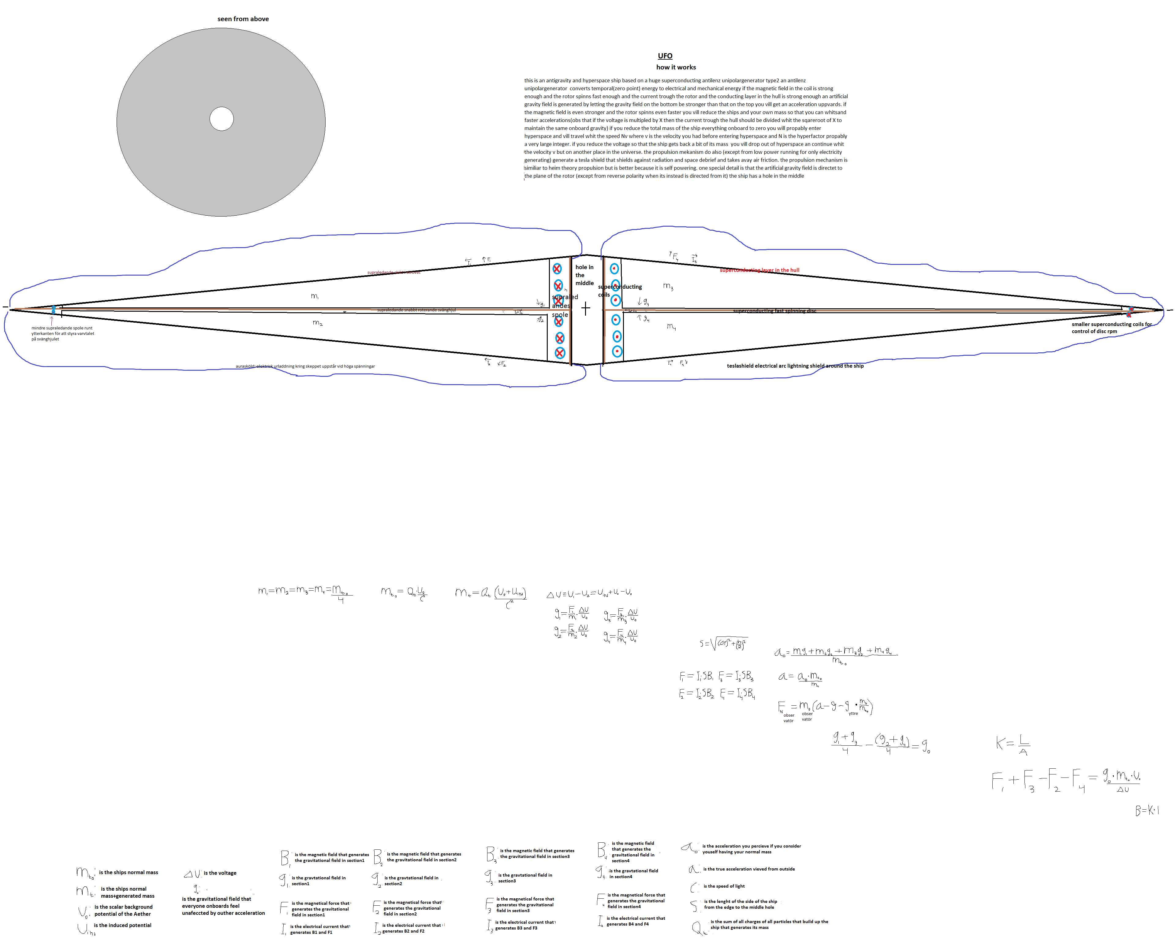